
This page carries the official NCERT Class 12 Physics Part I, Chapter 4, Moving Charges and Magnetism — the moving charges and magnetism class 12 chapter from the current edition, about 29 printed pages. The chapter PDF published by NCERT is linked below, followed by a guide to what is inside it, all maintained for the 2026-27 academic session.
Download the Moving Charges and Magnetism Class 12 NCERT PDF
Download the official Moving Charges and Magnetism Class 12 NCERT PDF straight from ncert.nic.in — the chapter exactly as printed in NCERT’s Physics Part I, with its figures, worked examples, section exercises and the chapter Summary in the book’s own pagination.
| What the chapter holds | Count | Where it is used |
|---|---|---|
| Printed pages | 29 | |
| Sections in the chapter | 15 | |
| Figures with NCERT captions | 23 | |
| Tables | 1 | |
| Worked examples | 5 | solved step by step in our NCERT Solutions |
| Exercise questions | 13 | answered in our NCERT Solutions |
| Official NCERT PDF | Download the chapter PDF | the chapter exactly as NCERT publishes it |
Chapter 4 at a Glance: What the PDF Contains
Chapter 4 is built in one direction: it establishes magnetic fields first, then forces on currents, then the instruments that use those forces.
- Sections 4.1–4.2 open with Oersted’s discovery, define the magnetic field and the Lorentz force, and extend the force to a current-carrying conductor.
- Section 4.3 follows one charged particle through circular and helical motion, and explains the cyclotron.
- Sections 4.4–4.5 reverse the question — how a current creates a field — answered by the Biot-Savart law and the circular loop.
- Sections 4.6–4.7 give Ampere’s circuital law as the symmetry shortcut and use it for a long wire and a solenoid.
- Section 4.8 derives the force between parallel currents and defines the ampere from it.
- Sections 4.9–4.10 show why a current loop feels a torque, and build the moving coil galvanometer on that torque.
- The chapter closes with a Summary, Points to Ponder and exercises.
The table below lists how much the chapter holds — sections, figures, worked examples and exercise questions — so you can gauge the file before opening it.
What This Chapter Teaches: Moving Charges Create Magnetism
The chapter does two jobs. First, moving charges and currents create magnetic fields around them. Second, magnetic fields exert forces and torques on moving charges and on current-carrying wires.
Both halves trace back to Oersted’s 1820 lecture demonstration: a compass needle deflected near a wire carrying current (NCERT, p. 108). The chapter then borrows the field idea from Chapter 1 — a charge sets up a field that acts on other charges; here a current sets up a magnetic field that acts on moving charges (NCERT, p. 109).
The book also adopts a drawing convention you must recognise before reading any diagram: a dot (\( \odot \)) marks a current or field coming out of the plane of the paper, a cross (\( \otimes \)) marks one going into it (NCERT, p. 108). Figure 4.1 in the walkthrough below shows both.
Lorentz Force and Magnetic Force on a Current-Carrying Wire
The Lorentz force is the chapter’s first building block: one expression for the total force on a charge \(q\) moving with velocity \(\mathbf{v}\) through an electric field \(\mathbf{E}\) and a magnetic field \(\mathbf{B}\) (NCERT, p. 109).
\[ \mathbf{F} = q(\mathbf{E} + \mathbf{v} \times \mathbf{B}) \]
The magnetic part \( q(\mathbf{v} \times \mathbf{B}) \) has three features worth testing yourself:
- It depends on \(q\), \(\mathbf{v}\) and \(\mathbf{B}\), and it reverses on a negative charge (NCERT, p. 109).
- It is zero when \(\mathbf{v}\) is parallel or antiparallel to \(\mathbf{B}\), because the cross product vanishes there.
- It is zero for a stationary charge — a magnetic field acts only on moving charge (NCERT, p. 109).
The same reasoning extends to a straight conductor. A rod of length \(l\) carrying current \(I\) in a field \(\mathbf{B}\) feels \( \mathbf{F} = I\,\mathbf{l} \times \mathbf{B} \), where the vector \(\mathbf{l}\) points along the current (NCERT, p. 110).
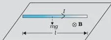
This setup is NCERT Example 4.1: the wire hangs in mid-air, so the upward magnetic force exactly balances gravity. Write the condition \( mg = IlB \), then solve for \(B\).
Worked example: the field that holds a wire in mid-air
Step 1: State the equilibrium.
For the wire to float without support, the magnetic force \(IlB\) must equal the weight \(mg\).
\[ B = \frac{mg}{Il} \]
Step 2: Use a wire of mass 120 g (0.12 kg), length 2.0 m, carrying 3 A.
\[ B = \frac{0.12 \times 9.8}{3 \times 2.0} = \frac{1.18}{6.0} \approx 0.20\ \text{T} \]
Final answer: \(B \approx 0.20\ \text{T}\). Only the mass per unit length matters, not the wire’s material (NCERT, p. 111).
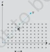
Direction is the catch in this chapter. With \(\mathbf{v}\) along +x and \(\mathbf{B}\) along +y, a proton is pushed along +z and an electron along −z — same rule, reversed answer (NCERT, p. 111, Example 4.2).
Motion in a Magnetic Field: Circular Paths, Helices and the Cyclotron
A magnetic field bends a moving charge without slowing it. The magnetic force is always perpendicular to the velocity, so it does no work and the speed never changes — only the direction does (NCERT, p. 112). The electric force \(q\mathbf{E}\) can do the opposite, because it can push along the motion.
When \(\mathbf{v}\) is perpendicular to a uniform \(\mathbf{B}\), the magnetic force acts as the centripetal force and the charge circles:
\[ r = \frac{mv}{qB}, \qquad \omega = \frac{qB}{m}, \qquad \nu_c = \frac{qB}{2\pi m} \]
Two results drive the cyclotron. The radius grows with momentum. And the frequency of revolution is independent of speed and radius (NCERT, p. 112), which lets the accelerating machine stay in step as particles gain energy.
If the velocity also has a component along \(\mathbf{B}\), that component is untouched, so the path becomes a helix. The distance advanced along the field in one turn is the pitch (NCERT, p. 113):
\[ p = v_{\parallel}T = \frac{2\pi m v_{\parallel}}{qB} \]
Worked example: a proton orbiting in a 0.5 T field
Step 1: Radius.
Use \( r = mv/(qB) \) with \(m = 1.67 \times 10^{-27}\ \text{kg}\), \(q = 1.6 \times 10^{-19}\ \text{C}\), \(v = 2 \times 10^{6}\ \text{m/s}\), \(B = 0.5\ \text{T}\).
\[ r = \frac{1.67 \times 10^{-27} \times 2 \times 10^{6}}{1.6 \times 10^{-19} \times 0.5} = \frac{3.34 \times 10^{-21}}{8.0 \times 10^{-20}} \approx 4.2 \times 10^{-2}\ \text{m} \]
Step 2: Frequency.
Use \( \nu = qB/(2\pi m) \).
\[ \nu = \frac{1.6 \times 10^{-19} \times 0.5}{2\pi \times 1.67 \times 10^{-27}} \approx 7.6 \times 10^{6}\ \text{Hz} \]
Final answer: radius \( \approx 4.2\ \text{cm} \), frequency \( \approx 7.6\ \text{MHz} \). Halving the speed would halve the radius but leave the frequency unchanged.
Biot-Savart Law and the Field of a Circular Current Loop
Here the question reverses: a current is given, find the field it produces. The Biot-Savart law is the magnetic analogue of Coulomb’s law — it gives the field contribution of a tiny current element (NCERT, p. 113).
\[ d\mathbf{B} = \frac{\mu_0}{4\pi}\frac{I\,d\mathbf{l} \times \mathbf{r}}{r^3}, \qquad |d\mathbf{B}| = \frac{\mu_0}{4\pi}\frac{I\,dl\sin\theta}{r^2} \]
The constant is \( \mu_0/4\pi = 10^{-7}\ \text{T m/A} \), and \(\mu_0\) is the permeability of free space (NCERT, p. 114). The total field of a finite wire comes from integrating every element’s contribution.
NCERT lists four contrasts with electrostatics (NCERT, p. 114). Both fields are inverse-square and obey superposition. But \(\mathbf{E}\) points along the displacement vector, while \(d\mathbf{B}\) is perpendicular to the plane of \(d\mathbf{l}\) and \(\mathbf{r}\).
The sources differ too: charge is a scalar source, a current element is a vector source. And Biot-Savart carries the factor \(\sin\theta\), which Coulomb’s law has no equivalent of — along the line of \(d\mathbf{l}\) itself, \(\theta = 0\) and the field is zero.
Integrating the law around a circular loop gives the field on its axis at distance \(x\), with the centre as the special case \(x = 0\) (NCERT, p. 116):
\[ B = \frac{\mu_0 I R^2}{2(x^2 + R^2)^{3/2}}, \qquad B_{\text{centre}} = \frac{\mu_0 I}{2R} \]
Worked example: centre and axial field of a 50-turn coil
Step 1: Centre field.
For \(N\) tightly wound turns, multiply the single-loop result by \(N\), the step NCERT Example 4.6 applies at the centre.
Use radius 5 cm (0.05 m), current 2 A, \(N = 50\).
\[ B = \frac{\mu_0 N I}{2R} = \frac{4\pi \times 10^{-7} \times 50 \times 2}{2 \times 0.05} \approx 1.26 \times 10^{-3}\ \text{T} \]
Step 2: Axial field at \(x = 15\ \text{cm}\).
Apply the same \(N\)-fold multiplication to \( B = \mu_0 I R^2/[2(x^2+R^2)^{3/2}] \).
\[ B = \frac{4\pi \times 10^{-7} \times 50 \times 2 \times (0.05)^2}{2(0.15^2 + 0.05^2)^{3/2}} \approx 4.0 \times 10^{-5}\ \text{T} \]
Final answer: \(1.26 \times 10^{-3}\ \text{T}\) at the centre, falling to \( \approx 4.0 \times 10^{-5}\ \text{T}\) at 15 cm on the axis. The field drops by a factor of about 30 over three radii of distance.
Ampere’s Circuital Law and the Magnetic Field of a Solenoid
Ampere’s circuital law is the symmetry shortcut — it replaces integration with a closed-loop integral. The line integral of \(\mathbf{B}\) around a loop equals \(\mu_0\) times the current passing through the surface bounded by that loop (NCERT, p. 118).
\[ \oint \mathbf{B} \cdot d\mathbf{l} = \mu_0 I \]
Most problems use the simplified form \( BL = \mu_0 I_e \). It works when, along the chosen Amperian loop, \(\mathbf{B}\) is tangential and constant, normal to the loop, or zero (NCERT, p. 118). A circle around a long straight wire is the classic case:
\[ B = \frac{\mu_0 I}{2\pi r} \]
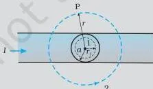
This cross-section view from NCERT Example 4.7 shows why the two regions differ. Outside the wire, the loop encloses all the current and \(B\) falls as \(1/r\). Inside, only the fraction of current inside the loop counts, and \(B\) grows linearly with \(r\) (NCERT, p. 120).
Know the limit of the law: it holds for any loop, but it is useful only where symmetry makes \(\mathbf{B}\) constant on the loop. NCERT is explicit that it cannot easily produce the centre field of a circular loop, \(B = \mu_0 I/2R\), because that geometry lacks the needed symmetry (NCERT, p. 120).
The solenoid is where the law pays off. A long solenoid has a uniform field inside and nearly zero outside, so the rectangular loop of Fig. 4.16 gives \(B\) directly in terms of \(n\), the turns per unit length (NCERT, p. 121):
\[ B = \mu_0 n I \]
Force Between Parallel Currents and the SI Definition of the Ampere
A current produces a field, and a field exerts a force on a current, so two wires side by side must push or pull each other. The field of conductor \(a\) acting on the current in conductor \(b\) gives the force per unit length (NCERT, p. 123):
\[ \frac{F}{L} = \frac{\mu_0 I_a I_b}{2\pi d} \]
Tracing the directions with the two right-hand rules gives the chapter’s most quoted result: parallel currents attract, and antiparallel currents repel (NCERT, p. 123). This is opposite to electrostatics, where like charges repel.
This force defines the SI unit of current. The ampere is the steady current that, maintained in each of two very long straight parallel conductors of negligible cross-section placed one metre apart in vacuum, produces a force of \(2 \times 10^{-7}\ \text{N}\) per metre on each (NCERT, p. 123).
The coulomb then follows: one coulomb is the charge that crosses a section in one second at one ampere.
Worked example: force between two parallel wires
Step 1: Two parallel wires carry 2 A and 3 A in the same direction, 10 cm apart.
Use \( F/L = \mu_0 I_a I_b/(2\pi d) \).
\[ \frac{F}{L} = \frac{4\pi \times 10^{-7} \times 2 \times 3}{2\pi \times 0.10} = 1.2 \times 10^{-5}\ \text{N/m} \]
Step 2: Decide the direction.
The currents run the same way, so the force is attractive.
Final answer: \(1.2 \times 10^{-5}\ \text{N}\) per metre, attractive. Reversing one current turns it into repulsion of the same magnitude.
Standardising the ampere is harder than the definition sounds. NCERT Example 4.9 shows that the earth’s field alone exerts about \(3 \times 10^{-5}\ \text{N/m}\) on a wire carrying 1 A — far larger than the \(2 \times 10^{-7}\ \text{N/m}\) being defined — so the earth’s field must be eliminated during calibration (NCERT, p. 124).
Torque on a Current Loop, Magnetic Moment and the Moving Coil Galvanometer
A current loop in a uniform field feels no net force, but it does feel a torque — the same behaviour as an electric dipole in a uniform electric field (NCERT, p. 125). The loop’s magnetic moment and the torque on it are (NCERT, pp. 126–127):
\[ \mathbf{m} = N I \mathbf{A}, \qquad \boldsymbol{\tau} = \mathbf{m} \times \mathbf{B} \]
The torque vanishes when \(\mathbf{m}\) is parallel or antiparallel to \(\mathbf{B}\), but the two equilibria differ. Parallel is stable — a small rotation produces a restoring torque. Antiparallel is unstable — any rotation grows (NCERT, p. 127).
The moving coil galvanometer converts this torque into a measurement. A radial field, produced by a cylindrical soft iron core, keeps the angle between coil and field fixed, so \(\sin\theta = 1\) is built in. The spring’s counter-torque balances the magnetic torque (NCERT, p. 130):
\[ k\phi = N I A B, \qquad \phi = \left(\frac{NAB}{k}\right) I \]
Because the deflection is proportional to the current, the scale is linear. Two sensitivities follow (NCERT, pp. 130–131):
- Current sensitivity \( \phi/I = NAB/k \) — the deflection per unit current.
- Voltage sensitivity \( \phi/V = (NAB/k)(1/R) \) — the deflection per unit voltage, with \(R\) the series resistance.
Conversion is a matter of resistance. A small shunt resistance in parallel makes an ammeter, letting most of the current bypass the coil. A large resistance in series makes a voltmeter, so the instrument draws almost no current (NCERT, pp. 130–131).
Doubling the turns \(N\) doubles the current sensitivity, but the coil’s resistance also doubles — it is proportional to wire length — so the voltage sensitivity is unchanged (NCERT, p. 131). NCERT Example 4.12 shows why the conversion matters: the bare galvanometer’s own resistance changed the very current it was meant to measure, while the shunted version read the true value.
Reading the Figures: A Walkthrough of NCERT’s Diagrams
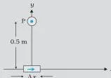
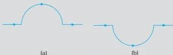
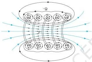
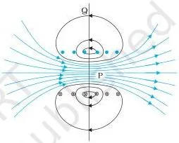
The figures in this chapter carry the physics — each one encodes a direction, a symmetry or a cancellation that the text assumes you can see. Work through them in book order.
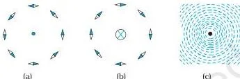
Read this figure in three parts. In (a) the current comes out of the page — the dot — and every needle points anticlockwise around the wire. In (b) the current goes in — the cross — and the needles reverse. Part (c) shows the same concentric field lines with iron filings (NCERT, p. 108).
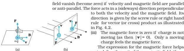
This is the rule for the cross product \(\mathbf{v} \times \mathbf{B}\): fingers sweep from \(\mathbf{v}\) to \(\mathbf{B}\), the thumb gives the force — for a positive charge. Part (b) is the trap: a negative charge deflects the other way. Ask the sign of the charge before you trust the thumb (NCERT, p. 110).
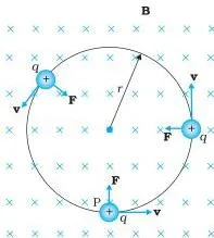
Here \(\mathbf{v}\) is perpendicular to \(\mathbf{B}\), and the magnetic force points to the centre at every instant — a perfect centripetal force. Equating \(qvB\) with \(mv^2/r\) gives the radius \(r = mv/qB\) (NCERT, p. 112).
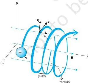
Add a velocity component along \(\mathbf{B}\) and the circle stretches into a helix. That component never changes, because the magnetic force has no component along the field. The spacing between turns is the pitch (NCERT, p. 113).
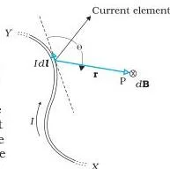
This is the geometry behind every Biot-Savart calculation. The element \(d\mathbf{l}\) and the displacement \(\mathbf{r}\) define a plane; \(d\mathbf{B}\) sticks out of that plane — here into the page, hence the cross. The magnitude carries the factor \(\sin\theta\), where \(\theta\) is the angle between \(d\mathbf{l}\) and \(\mathbf{r}\) (NCERT, p. 113).
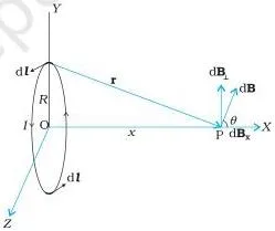
This figure explains the integration trick. Every element contributes a \(d\mathbf{B}\) tilted relative to the axis, but the perpendicular components from opposite elements cancel in pairs. Only the axial components survive, and summing them around the loop gives the axial field formula (NCERT, pp. 115–116).
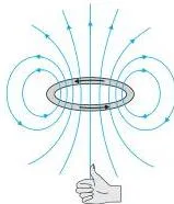
Two things to notice. The field lines are closed loops passing through the coil — magnetic field lines never begin or end. And the loop behaves like a bar magnet, with one face a north pole and the other a south pole, which is why a current loop is called a magnetic dipole (NCERT, p. 116).
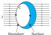
Ampere’s law connects the boundary of a surface to what passes through it: the line integral of \(\mathbf{B}\) along the boundary equals \(\mu_0\) times the current threading the surface. The right-hand rule fixes which direction of current counts as positive (NCERT, pp. 117–118).
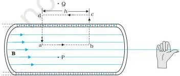
Only side \(ab\) of the rectangle contributes: \(cd\) lies outside where the field is zero, and the two transverse sides have \(\mathbf{B}\) perpendicular to them. If \(h\) is the length of \(ab\), the loop encloses \(nh\) turns, and the law gives \(Bh = \mu_0 (nhI)\), hence \(B = \mu_0 n I\) (NCERT, p. 121).
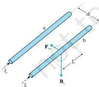
Follow the two steps in order. Conductor \(a\) sets up the field \(B_a\) at the position of \(b\); that field then exerts a force on the current in \(b\). For currents in the same direction the force on \(b\) points toward \(a\), and by Newton’s third law the force on \(a\) points toward \(b\) (NCERT, pp. 122–123).
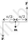
The field lies in the plane of the coil here. Arms AD and BC feel no force, while arms AB and CD feel equal and opposite forces that are not collinear — a couple. Net force zero, net torque \(IAB\), which is why the coil rotates instead of translating (NCERT, p. 125).
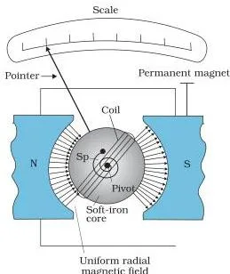
The cylindrical soft iron core does two jobs: it makes the field radial, keeping the torque at full strength for every deflection, and it strengthens the field. The spring then balances the magnetic torque, so the pointer stops at an angle proportional to the current: \(k\phi = NIAB\) (NCERT, p. 130).
Key Definitions in Chapter 4
These terms return in later chapters, so define each one once, in your own words. The page numbers point to where the book introduces them.
| Term | Plain definition | NCERT page |
|---|---|---|
| Magnetic field \(\mathbf{B}\) | Vector field set up by moving charges and currents that exerts a force on other moving charges | p. 109 |
| Tesla | SI unit of magnetic field — the field that gives a force of 1 N on a 1 C charge moving at 1 m/s perpendicular to it | pp. 109–110 |
| Gauss | Non-SI unit of magnetic field, equal to \(10^{-4}\ \text{T}\), convenient for small fields | p. 110 |
| Lorentz force | Total force on a charge moving through electric and magnetic fields: \( \mathbf{F} = q(\mathbf{E} + \mathbf{v} \times \mathbf{B}) \) | p. 109 |
| Cyclotron frequency | Frequency of revolution of a charge circling in a uniform field, \( \nu = qB/2\pi m \), independent of speed and radius | p. 112 |
| Pitch | Distance a particle advances along the field in one turn of its helix, \( p = v_{\parallel}T \) | p. 113 |
| Permeability of free space \( \mu_0 \) | Constant linking current to the field it produces in vacuum; \( \mu_0/4\pi = 10^{-7}\ \text{T m/A} \) | p. 114 |
| Magnetic moment \( \mathbf{m} \) | For a planar loop, magnitude \(NIA\) directed by the right-hand thumb rule; unit \( \text{A m}^2 \) | p. 126 |
| Shunt resistance | Small resistance in parallel with a galvanometer coil so most of the current bypasses the coil | p. 130 |
| Current sensitivity | Deflection per unit current in a galvanometer, \( \phi/I = NAB/k \) | p. 130 |
| Voltage sensitivity | Deflection per unit voltage, \( \phi/V = (NAB/k)(1/R) \) | p. 131 |
Common Mistakes in Moving Charges and Magnetism
Most errors in this chapter are directional, not numerical — the number comes out right and the direction is backwards. The table names the errors before you make them.
| Mistake | Correct rule | How to check your answer |
|---|---|---|
| Using the right-hand rule for a positive charge and forgetting the electron | The force on a negative charge is opposite to that on a positive charge (NCERT, p. 110) | Work the rule for a proton first, then reverse the direction; Example 4.2’s +z and −z pair is the model |
| Thinking a magnetic field can speed a particle up or slow it down | The magnetic force is always perpendicular to \( \mathbf{v} \), so it does no work and speed stays constant (NCERT, p. 112) | Check whether the force has any component along the velocity — it never does |
| Confusing the two right-hand rules | Straight wire: thumb along the current, fingers curl along \( \mathbf{B} \). Loop: fingers curl along the current, thumb points along \( \mathbf{B} \) on the axis (NCERT, p. 119, footnote) | Name the situation first — in the wire rule the current is in the thumb; in the loop rule the current is in the fingers |
| Assuming like currents repel because like charges repel | Parallel currents attract; antiparallel currents repel (NCERT, p. 123) | Draw the field of wire a at wire b, then apply \( \mathbf{F} = I\,\mathbf{l} \times \mathbf{B} \); the pull or push falls out |
| Applying Ampere’s law where symmetry does not make \( \mathbf{B} \) constant | The simplified form \( BL = \mu_0 I_e \) needs \( \mathbf{B} \) tangential and constant on the loop; the centre of a circular loop lacks this (NCERT, p. 120) | Ask whether \( \mathbf{B} \) wraps a candidate loop with the same magnitude everywhere; if not, use Biot-Savart |
| Mixing up stable and unstable equilibrium of \( \mathbf{m} \) with \( \mathbf{B} \) | \( \mathbf{m} \) parallel to \( \mathbf{B} \) is stable (rotation restores); antiparallel is unstable (rotation grows) (NCERT, p. 127) | Tilt the coil slightly and ask whether the torque pulls it back or pushes it further |
One more from Points to Ponder: magnetic field lines always form closed loops, unlike electric field lines, which start on positive charges and end on negative ones. Any sketch you draw must close on itself (NCERT, p. 134).
Exam Notes: How to Revise This Chapter
Start with the chapter’s own examples and exercises — they are the question bank. Work each numerical fully: substitution with units, the calculation, and a final statement of magnitude and direction.
The exercise set maps to concepts like this:
- Fields of coils and straight wires — Exercises 4.1 and 4.2 are direct formula applications; 4.3 and 4.4 add direction, so the answer must give magnitude, direction and the rule used.
- Forces on wires — Exercises 4.5 (wire at an angle to \( \mathbf{B} \)) and 4.6 (wire inside a solenoid) test \( F = BIl\sin\theta \); Exercise 4.7 is the parallel-wire force.
- Solenoid field — Exercise 4.8 stacks several layers of windings; find the total turns per unit length before substituting.
- Torque on coils — Exercises 4.9 and 4.13 use \( \tau = NIAB\sin\theta \); 4.13(b) asks the conceptual question of whether the coil’s shape matters.
- Galvanometer sensitivity — Exercise 4.10 compares the current and voltage sensitivity of two moving coil meters.
- Circular motion of an electron — Exercises 4.11 and 4.12 ask you to explain why the path is circular, then compute radius and frequency, and state whether the frequency depends on speed.
For each right-hand rule, practise one direction problem: sketch \( \mathbf{v} \), \( \mathbf{B} \) and \( \mathbf{F} \) for a positive and a negative charge, then repeat for a straight wire and for a loop. If you can name the rule you used, you own the concept.
Textbook contents and the examinable syllabus are not always identical — check the current official CBSE syllabus before you decide what to revise.
Moving Charges and Magnetism: The Chapter in Ten Points
This digest is built from the chapter’s own Summary (NCERT, pp. 132–133), rewritten in plainer words — ten results worth recalling the night before.
- The Lorentz force \( \mathbf{F} = q(\mathbf{E} + \mathbf{v} \times \mathbf{B}) \) is the total force on a moving charge; its magnetic part does zero work because it is normal to \( \mathbf{v} \).
- A straight conductor of length \(l\) carrying current \(I\) in field \( \mathbf{B} \) feels \( \mathbf{F} = I\,\mathbf{l} \times \mathbf{B} \).
- A charge circles in a plane normal to \( \mathbf{B} \) with \( r = mv/qB \); the cyclotron frequency \( qB/2\pi m \) is independent of speed — the idea behind the cyclotron.
- The Biot-Savart law \( d\mathbf{B} = (\mu_0/4\pi)\, I\,d\mathbf{l} \times \mathbf{r}/r^3 \) gives the field of a current element; integrate over the whole conductor for the total field.
- A circular coil of radius \(R\) gives \( B = \mu_0 I R^2/[2(x^2+R^2)^{3/2}] \) on its axis, reducing to \( \mu_0 I/2R \) at the centre.
- Ampere’s circuital law \( \oint \mathbf{B}\cdot d\mathbf{l} = \mu_0 I \) is the symmetry shortcut; in simplified form, \( BL = \mu_0 I_e \).
- A long straight wire gives \( B = \mu_0 I/2\pi r \), with field lines that are concentric circles.
- Inside a long solenoid, \( B = \mu_0 n I \), uniform and parallel to the axis.
- Parallel currents attract; antiparallel currents repel.
- A planar loop has magnetic moment \( \mathbf{m} = NI\mathbf{A} \); in a uniform field it feels \( \boldsymbol{\tau} = \mathbf{m} \times \mathbf{B} \), which the galvanometer balances with a spring, \( k\phi = NIAB \). A shunt in parallel makes an ammeter; a large series resistance makes a voltmeter.
Two cautions close the chapter’s Points to Ponder. Everything above assumes steady currents that do not vary with time. And Ampere’s law is not independent of the Biot-Savart law — it can be derived from it (NCERT, p. 134).
Related Resources: Class 12 Physics Chapters
Chapter 4 sits in the first half of NCERT Class 12 Physics Part I, between Current Electricity and the magnetism chapters. Use these links to move around the book and the site.
- Class 12 Physics notes — the hub for this subject, where the previous chapter, Current Electricity, also lives.
- Magnetism and Matter (Chapter 5) notes — the next chapter, which builds on the magnetic dipole idea introduced here.
- Dual Nature of Radiation and Matter notes — a later chapter in the same book that studies the motion of charged particles.
- Class 12 study resources — notes across subjects for the same class.
- CBSE notes home — the starting point for any class or subject.
The official textbook portal carries the full book: NCERT Class 12 Physics textbooks and other titles on ncert.nic.in.
Sources and Data Verification
The contents described on this page are from NCERT Class 12 Physics Part I, Chapter 4, Moving Charges and Magnetism, in the official edition published by NCERT and available on ncert.nic.in.
- Figure captions, page numbers and quoted results come from this printed textbook edition; page references match the book’s own pagination.
- This page covers Chapter 4 of Physics Part I only — not the rest of the book, and not the wider CBSE scheme.
- NCERT settles textbook editions and PDFs. CBSE settles curriculum, syllabus and examinations.
- A chapter appearing in the textbook does not by itself prove every part of it is examinable this session — check the current official syllabus.
- No external review process is claimed for this page.
Reference: NCERT Class 12 Physics textbook, chapter 4, official edition on ncert.nic.in.
Frequently Asked Questions About Moving Charges and Magnetism
Why does a magnetic field not change the speed of a moving charged particle?
The magnetic force \( q(\mathbf{v} \times \mathbf{B}) \) is always perpendicular to the velocity, so it never has a component along the motion. A force perpendicular to displacement does no work, and work is what changes speed. So the field changes the direction of the velocity but never its magnitude (NCERT, p. 112).
Why do two parallel currents attract each other while opposite currents repel?
Conductor \(a\) sets up a magnetic field at the position of conductor \(b\), and that field exerts a force on the current in \(b\). Apply the two right-hand rules in order — the field of \(a\), then the force on \(b\). For currents in the same direction the force on \(b\) points toward \(a\).
Newton’s third law then pulls \(a\) toward \(b\). Reversing one current reverses the field it produces, and the attraction becomes a repulsion (NCERT, p. 123).
What is the difference between the Biot-Savart law and Ampere’s circuital law?
They express the same physics in two ways. The Biot-Savart law adds the field of every current element, so it works for any conductor shape, but the integration can be heavy. Ampere’s law integrates \( \mathbf{B} \) around a closed loop and equates it to \( \mu_0 \) times the enclosed current.
Ampere’s law is much faster, but genuinely useful only when symmetry makes \( \mathbf{B} \) constant on the loop, as for a straight wire or a solenoid. The chapter notes that Ampere’s law is not independent of Biot-Savart; it can be derived from it (NCERT, pp. 117–118, 134).
Why does doubling the number of turns in a galvanometer not double its voltage sensitivity?
Current sensitivity, \( \phi/I = NAB/k \), doubles with \(N\) because the torque per unit current doubles. But voltage sensitivity is \( \phi/V = (NAB/k)(1/R) \), and the coil’s resistance is proportional to the length of its wire.
So doubling \(N\) doubles \(R\) as well, and the two factors cancel: \(2N\) together with \(2R\) leaves \( \phi/V \) unchanged (NCERT, p. 131).
Is the cyclotron frequency of a charged particle independent of its speed?
Yes. The frequency is \( \nu = qB/2\pi m \), which contains neither the speed nor the radius (NCERT, p. 112). As a particle gains energy in a cyclotron and its orbit grows, its revolution frequency does not change, which is what makes the machine’s design possible.
Explore Class 12 Physics Books
Class 12 Physics on LearnCBSE:
Related chapters: