
Magnetism and Matter Class 12 is Chapter 5 of the NCERT Class 12 Physics Part I textbook: an 18-page chapter running from page 135 to page 153 of the 2026-27 edition. The official NCERT chapter PDF is offered right here, followed by a guide to what each section teaches — bar magnets, Gauss’s law, and magnetic materials.
Download the Magnetism and Matter Class 12 Chapter PDF
The official file is Chapter 5 of the Physics Part I textbook for Class 12, hosted by NCERT itself, and it is the same file your school’s copy is printed from.
Open the NCERT Class 12 Physics Chapter 5 Magnetism and Matter PDF to read the chapter exactly as NCERT prints it, with every figure, table and exercise in place — the page numbers cited in this guide follow that printed pagination.
If the chapter file ever fails to open, use the official index page for Physics Part I on ncert.nic.in; it lists every chapter file in the book, so you can verify the edition or jump straight to Chapter 4 or Chapter 6.
| What the chapter holds | Count | Where it is used |
|---|---|---|
| Printed pages | 18 | |
| Sections in the chapter | 12 | |
| Figures with NCERT captions | 9 | |
| Tables | 3 | |
| Worked examples | 2 | solved step by step in our NCERT Solutions |
| Exercise questions | 7 | answered in our NCERT Solutions |
| Official NCERT PDF | Download the chapter PDF | the chapter exactly as NCERT publishes it |
Chapter at a Glance: What Is Inside This Chapter
Use the block below to see how Chapter 5 is organised — its sections, figures, worked examples and exercise questions — before you decide where to spend your revision time.
What This Chapter Covers: From Bar Magnets to Magnetic Materials
Chapter 4 treated magnetism as an effect of electric currents; this chapter takes magnetism as a subject in its own right (NCERT, p. 135). It starts from the object you already know — the bar magnet — and builds a complete description of magnetic fields, the energy of a dipole in a field, and why materials respond to magnets as they do.
In reading order, the chapter moves through seven ideas:
- The bar magnet and its field lines — how to picture a dipole with iron filings or a compass (p. 137).
- The bar magnet as an equivalent solenoid — circulating currents explain every magnetic effect (p. 138).
- Torque and potential energy of a magnetic dipole in a uniform field (p. 139).
- The electrostatic analog — replace p by m and electric results become magnetic ones (p. 140-141).
- Gauss’s law of magnetism — net magnetic flux through any closed surface is zero (p. 142-144).
- Magnetisation and magnetic intensity — the B, H and M relations that classify materials (p. 145-146).
- The three classes of magnetic materials — diamagnetic, paramagnetic and ferromagnetic (p. 147-149).
The chapter closes with a summary, a table of physical quantities, points to ponder and seven exercises (p. 149-153). None of that needs formulas to be introduced; the sections below decode every equation one symbol at a time.
The Bar Magnet: Field Lines, Poles and the Dipole Idea
A bar magnet is the chapter’s starting object, and its behaviour gives the field-line picture everything else uses. Suspend a bar magnet freely and it settles pointing north-south; the end pointing to the geographic north is called the north pole, the other the south pole (NCERT, p. 135).
Sprinkle iron filings on a glass sheet over a bar magnet and they arrange themselves along curved lines — the pattern of Fig. 5.1, which is the signature of a magnetic dipole (NCERT, p. 137). Magnetic field lines have four properties, and every later argument in the chapter leans on them (NCERT, p. 137-138):
- They form continuous closed loops — unlike electric dipole lines, which begin on positive charge and end on negative charge or escape to infinity.
- The tangent to a field line at any point gives the direction of the net magnetic field B there.
- The more crowded the lines, the stronger the field — in Fig. 5.2(a) the field is stronger around region (ii) than region (i).
- They never intersect — at a crossing the direction of B would not be unique.
The book adds a warning in a footnote: calling field lines “lines of force” is misleading, because the magnetic force on a moving charge is perpendicular to B, not along the line (NCERT, p. 137). A compass needle moved point by point plots the same pattern as iron filings.
Bar Magnet as an Equivalent Solenoid
Why can a permanent magnet be modelled as a coil of wire? Because every magnetic field is produced by moving charges. The chapter closes Chapter 4’s argument that a current loop acts as a magnetic dipole and recalls Ampere’s hypothesis that all magnetic phenomena can be explained by circulating currents (NCERT, p. 138).
Cut a solenoid in half and you get two weaker solenoids; cut a bar magnet in half and you get two weaker magnets. The field lines stay continuous, emerging from one face and entering the other.
That resemblance is made quantitative by calculating the axial field of a finite solenoid (Fig. 5.3(a)) and showing it matches the far axial field of a bar magnet.
The axial-field formula (Eq. 5.1, NCERT p. 139): at a distance r from the centre, with r much larger than the object’s size, the field magnitude is \[ B = \frac{\mu_0}{4\pi}\frac{2m}{r^3} \]
Symbols: \( \mu_0 = 4\pi \times 10^{-7}\ \text{T m A}^{-1} \) is the permeability of free space; \( m \) is the magnetic moment in \( \text{A m}^2 \); \( r \) is the distance from the centre in metres.
The formula holds only for \( r \) much larger than the magnet’s size.
So a bar magnet of moment m produces the same far field as a solenoid of the same moment — the book states plainly that a bar magnet and a solenoid produce similar magnetic fields, and that the magnetic moment of the bar magnet equals that of the equivalent solenoid (NCERT, p. 139).
Torque and Potential Energy in a Uniform Magnetic Field
A uniform magnetic field does not push a needle anywhere — it rotates it. That distinction between force and torque drives this whole section.
The torque on a magnetic dipole m in a uniform field B is (Eq. 5.2, NCERT p. 139):
\[ \boldsymbol{\tau} = \mathbf{m}\times\mathbf{B}, \qquad \tau = mB\sin\theta \]
where \( \theta \) is the angle between m and B. Because it is a cross product, the torque is maximum when the moment is perpendicular to the field (\(\theta = 90^\circ\)) and zero when it is parallel or anti-parallel. Alongside this, the net force on a dipole in a uniform field is zero — the field turns the needle but never drags it.
The potential energy comes from integrating the torque (Eq. 5.3, NCERT p. 139):
\[ U_m = -\mathbf{m}\cdot\mathbf{B} = -mB\cos\theta \]
Three behavioural facts follow, and they are a favourite trap:
- The zero of potential energy is fixed at \(\theta = 90^\circ\) — the book chooses the constant of integration so the energy is zero when the needle is perpendicular to the field.
- At \(\theta = 0^\circ\) (aligned with B), \( U = -mB \), the minimum — this is stable equilibrium.
- At \(\theta = 180^\circ\) (anti-aligned), \( U = +mB \), the maximum — unstable equilibrium.
Worked example (fresh values): a magnetic needle of moment \( 1.2\ \text{A m}^2 \) makes an angle of \( 40^\circ \) with a uniform \( 0.6\ \text{T} \) field.
- Step 1: Write the data in SI units: \( m = 1.2\ \text{A m}^2 \), \( B = 0.6\ \text{T} \), \( \theta = 40^\circ \).
- Step 2: Torque: \( \tau = mB\sin\theta = 1.2 \times 0.6 \times \sin 40^\circ \).
\[ \tau = 0.72 \times 0.6428 \approx 0.46\ \text{N m} \]
Step 3: Potential energy: \( U = -mB\cos\theta = -1.2 \times 0.6 \times \cos 40^\circ \).
\[ U = -0.72 \times 0.7660 \approx -0.55\ \text{J} \]
Final answer: the needle feels a torque of about \( 0.46\ \text{N m} \) rotating it toward alignment, and its potential energy in this orientation is about \( -0.55\ \text{J} \).
The same section answers an everyday puzzle (Example 5.1(b), NCERT p. 140): an iron nail near a bar magnet is attracted even though the field is non-uniform.
The nail gains an induced moment, and the induced pole nearer the magnet is always the opposite pole — the induced south pole sits closer to the magnet’s north pole than the induced north pole does, so attraction wins.
The Electrostatic Analog: Turning p into m
This is the shortcut that makes the rest of the chapter easy: everything you already know about electric dipoles transfers to magnets with three replacements (NCERT p. 140).
- E → B — electric field becomes magnetic field.
- p → m — electric dipole moment becomes magnetic moment.
- \( \frac{1}{4\pi\varepsilon_0} \to \frac{\mu_0}{4\pi} \) — the Coulomb constant becomes the magnetic constant.
For a short magnet of size l, at distance r much larger than l, the two field expressions are Eqs. 5.4 and 5.5 (NCERT p. 140):
\[ \mathbf{B}_E = -\frac{\mu_0 \mathbf{m}}{4\pi r^3} \quad \text{(equatorial field)} \]
\[ \mathbf{B}_A = \frac{\mu_0}{4\pi}\frac{2\mathbf{m}}{r^3} \quad \text{(axial field)} \]
The equatorial field is negative — it points opposite to m — and the axial field is twice its magnitude. The axial expression is simply Eq. 5.1 in vector form. Table 5.1 in the book (p. 141) carries the whole analogy in one place:
| Quantity | Electrostatics | Magnetism |
|---|---|---|
| Dipole moment | \( \mathbf{p} \) | \( \mathbf{m} \) |
| Equatorial field (short dipole) | \( -\dfrac{p}{4\pi\varepsilon_0 r^3} \) | \( -\dfrac{\mu_0 m}{4\pi r^3} \) |
| Axial field (short dipole) | \( \dfrac{2p}{4\pi\varepsilon_0 r^3} \) | \( \dfrac{\mu_0 2m}{4\pi r^3} \) |
| Torque in external field | \( \mathbf{p}\times\mathbf{E} \) | \( \mathbf{m}\times\mathbf{B} \) |
| Energy in external field | \( -\mathbf{p}\cdot\mathbf{E} \) | \( -\mathbf{m}\cdot\mathbf{B} \) |
Hear the conversion once and it stays with you: the electric axial field \( \frac{2p}{4\pi\varepsilon_0 r^3} \) becomes the magnetic axial field \( \frac{\mu_0 2m}{4\pi r^3} \). Exercise 5.7 is nothing but these two formulas applied.
Gauss’s Law of Magnetism: Zero Net Flux, No Magnetic Monopoles
Wrap any closed surface around the end of a bar magnet and ask: how much magnetic flux leaves it? Because field lines form closed loops, every line that enters the surface must also leave it — so the net flux is zero. That single thought is Gauss’s law for magnetism.
The book builds it carefully. For a small vector area element \( \Delta\mathbf{S} \) of a closed surface S, the magnetic flux through it is \( \Delta\phi_B = \mathbf{B}\cdot\Delta\mathbf{S} \) (Fig. 5.5, NCERT p. 142). Sum over all area elements of the closed surface (Eq. 5.6, NCERT p. 142):
\[ \phi_B = \sum_{\text{all}} \mathbf{B}\cdot\Delta\mathbf{S} = 0 \]
Compare electrostatics, where the same sum equals \( q/\varepsilon_0 \), the charge enclosed. Magnetic flux has no such source term because there is no magnetic charge to enclose (NCERT p. 142-143).
The consequence is stated plainly: isolated magnetic poles, called monopoles, are not known to exist. The simplest magnetic element is a dipole or a current loop, and all magnetic phenomena can be explained as arrangements of dipoles and current loops (NCERT p. 143).
Two test cases from Example 5.1 make the point: a toroid has zero net magnetic moment and therefore has no poles, and neither does a straight infinite conductor (Example 5.1(c), NCERT p. 140). In Fig. 5.2(a) and (b), the closed Gaussian surfaces marked (i) and (ii) each capture equal numbers of entering and leaving lines — the visual form of the law.
Magnetisation and Magnetic Intensity: The B, H and M Relations
To classify materials, the chapter needs quantities that separate “what the solenoid does” from “what the material does”. Magnetic intensity H describes the external cause; magnetisation M describes the material’s response.
Definitions in order (NCERT p. 145-146):
- Magnetisation \( \mathbf{M} = \mathbf{m}_{\text{net}}/V \) — net magnetic moment per unit volume (Eq. 5.7). Vector, unit \( \text{A m}^{-1} \).
- Empty solenoid: \( B_0 = \mu_0 n I \) — interior field of a long solenoid with n turns per metre carrying current I (Eq. 5.8).
- With a material core, the total field is \( B = B_0 + B_m \), where the core contributes \( B_m = \mu_0 M \) (Eqs. 5.9 and 5.10).
- Magnetic intensity \( H = B/\mu_0 – M \) (Eq. 5.11), unit \( \text{A m}^{-1} \) — same unit as M. Rearranged: \( B = \mu_0(H + M) \) (Eq. 5.12).
- Linear materials obey \( M = \chi H \) (Eq. 5.13), where \( \chi \) is the magnetic susceptibility — small and positive for paramagnetic, small and negative for diamagnetic.
- The chain finishes with \( \mu_r = 1 + \chi \), \( \mu = \mu_0\mu_r \), so \( B = \mu H \) (Eqs. 5.14 and 5.15).
Worked example (fresh values, modelled on Example 5.5): a solenoid has 500 turns per metre and carries 1.5 A; its core material has relative permeability 200.
- Step 1: H depends only on the solenoid, not on the core: \( H = nI = 500 \times 1.5 = 750\ \text{A m}^{-1} \).
- Step 2: \( B = \mu_r\mu_0 H = 200 \times (4\pi \times 10^{-7}) \times 750 \).
\[ B \approx 0.19\ \text{T} \]
Step 3: \( M = (\mu_r – 1)H = 199 \times 750 \).
\[ M \approx 1.5 \times 10^5\ \text{A m}^{-1} \]
Final answer: \( H = 750\ \text{A m}^{-1} \), \( B \approx 0.19\ \text{T} \), \( M \approx 1.5 \times 10^5\ \text{A m}^{-1} \). Magnetisation is huge compared with H because the core multiplies the effect 199 times over.
Diamagnetic, Paramagnetic and Ferromagnetic Materials
The one-line rule is the sign and size of \( \chi \): negative means diamagnetic, small positive means paramagnetic, large positive means ferromagnetic (NCERT p. 147). The physics behind each class explains why.
Diamagnetism
Diamagnetic atoms have zero net magnetic moment (NCERT p. 147-148). An applied field acts on the orbiting electrons; in line with Lenz’s law — studied properly in Chapter 6 — electrons whose orbital moments point along the field slow down and those opposite speed up. The material therefore develops an induced moment opposite to the field, so it is repelled from strong field.
The effect is universal, present in all substances, but weak — about one part in \( 10^5 \). Book examples: bismuth, copper, lead, silicon, nitrogen (at STP), water and sodium chloride.
Paramagnetism
Paramagnetic atoms carry a permanent dipole moment of their own (NCERT p. 148). Random thermal motion keeps these moments unaligned, so there is no net magnetisation. A strong external field at low temperature aligns them partially with \( B_0 \), and the material is weakly attracted toward strong field. The enhancement is again about one part in \( 10^5 \).
Book examples: aluminium, sodium, calcium, oxygen (at STP) and copper chloride.
Ferromagnetism
Ferromagnetic atoms align spontaneously over macroscopic regions called domains — about 1 mm across, each containing roughly \( 10^{11} \) atoms (NCERT p. 149). An external field grows the domains aligned with it and rotates the others into them, until a single giant domain forms and the material is strongly attracted. Elements: iron, cobalt, nickel and gadolinium, with relative permeability above 1000.
Materials that keep their magnetisation after the field is removed — alnico and the naturally occurring lodestone — are hard ferromagnets, used for permanent magnets; soft iron, which loses its magnetisation, is a soft ferromagnet.
| Property | Diamagnetic | Paramagnetic | Ferromagnetic |
|---|---|---|---|
| Susceptibility \( \chi \) | small and negative (\( -10^{-5} \)) | small and positive (\( +10^{-5} \)) | large and positive |
| Range of \( \chi \) (Table 5.2) | \( -1 \le \chi \lt 0 \) | \( 0 \lt \chi \lt \varepsilon \) (tiny) | \( \chi \gg 1 \) |
| Relative permeability \( \mu_r \) | \( 0 \le \mu_r \lt 1 \) | \( 1 \lt \mu_r \lt 1 + \varepsilon \) | \( \mu_r \gg 1 \) (above 1000) |
| \( \mu \) vs \( \mu_0 \) | \( \mu \lt \mu_0 \) | \( \mu \gt \mu_0 \) | \( \mu \gg \mu_0 \) |
| Motion in a non-uniform field | strong → weak (repelled) | weak → strong (weakly attracted) | weak → strong (strongly attracted) |
| Book’s examples | bismuth, copper, lead, silicon, nitrogen, water, sodium chloride | aluminium, sodium, calcium, oxygen, copper chloride | iron, cobalt, nickel, gadolinium; alnico and lodestone (hard), soft iron (soft) |
Two more facts complete the picture. Superconductors are perfect diamagnets: at very low temperatures they expel the field completely, with \( \chi = -1 \) and \( \mu_r = 0 \), a phenomenon called the Meissner effect (NCERT p. 148). A superconductor repels a magnet and is repelled by it, which is the principle behind magnetically levitated superfast trains.
And temperature breaks ferromagnetism: at high enough temperature a ferromagnet becomes a paramagnet as the domain structure disintegrates, and the disappearance is gradual (NCERT p. 149).
How to Read the Figures in This Chapter
Every diagram in this chapter carries a piece of the argument. The walkthrough below reads them one by one, so a figure you might glance past in the book becomes a summary you can recall.
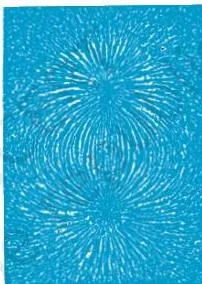
The filings line up end to end along the field, densest near the poles where the field is strongest. The pattern is the signature of a dipole: lines leave one pole, curve round, and enter the other (NCERT p. 137).
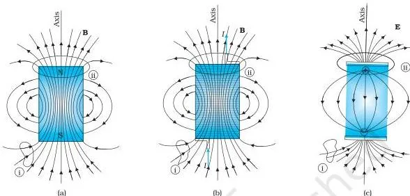
This is the chapter’s key comparison. At large distances the three patterns look alike, but magnetic lines close on themselves while electric lines end on charges. The surfaces (i) and (ii), drawn over the magnetic patterns, capture equal numbers of entering and leaving lines — the visual basis of Gauss’s law (NCERT p. 138, p. 142).
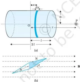
Part (a) is the geometry behind Eq. 5.1 — the axial field that matches a bar magnet’s. Part (b) defines the angle \( \theta \) between m and B, the angle in \( \tau = mB\sin\theta \) and \( U = -mB\cos\theta \) (NCERT p. 138-139).
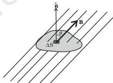
The figure accompanies the flux argument: split the closed surface S into small area elements \( \Delta\mathbf{S} \), define the flux through each as \( \Delta\phi_B = \mathbf{B}\cdot\Delta\mathbf{S} \), and sum over all elements — Eq. 5.6 gives zero (NCERT p. 142).
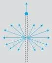
This is the chapter’s spot-the-error gallery (Example 5.3, NCERT p. 143-144). The verdicts, with one-line reasons:
- (a) Wrong. Lines can never emanate from a single point; that pattern is the electric field of a long charged wire.
- (b) Wrong. Lines can never cross (direction would be ambiguous), and a static magnetic loop must enclose a current — never empty space.
- (c) Right. Toroid: every closed loop encloses the windings carrying current.
- (d) Wrong. Solenoid field lines cannot be perfectly straight and confined outside the ends; they must curve out and close, else Ampere’s law is violated.
- (e) Right. Bar magnet, inside and out — note the lines inside run from S to N, and net flux around either pole is zero.
- (f) Wrong. Lines appear to emanate from a shaded plate, giving non-zero net flux — impossible for magnetism; it is the electric field between charged plates.
- (g) Wrong. Lines between pole pieces can never be exactly straight at the ends — some fringing is inevitable.
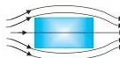
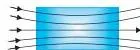
The pair is the visual mnemonic for the whole classification (NCERT p. 147-148): lines avoid a diamagnet and crowd through a paramagnet. In both cases the change is slight — about one part in \( 10^5 \).
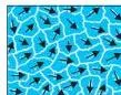
This figure carries the chapter’s warning that closes the ferromagnetism section (NCERT p. 149): at high enough temperature a ferromagnet becomes a paramagnet, because the domain structure disintegrates — and the disappearance is gradual.
The same page uses Fig. 5.8(a) and (b) to show the mechanism: randomly oriented domains with no bulk magnetisation, then the aligned single giant domain once an external field is applied.
Key Definitions: The Physical Quantities of Magnetism
The chapter’s closing table of physical quantities (NCERT p. 151) collects every new quantity with its symbol, dimensions and SI unit — the fastest way to check a definition before a numerical. This glossary reproduces it in plain words.
| Quantity | What it means | Symbol | SI unit |
|---|---|---|---|
| Permeability of free space | the constant fixing the strength of magnetic effects in vacuum; \( \mu_0/4\pi = 10^{-7} \) | \( \mu_0 \) | \( \text{T m A}^{-1} \) |
| Magnetic field (induction, flux density) | the magnetic field itself; \( 10^4\ \text{G (gauss)} = 1\ \text{T} \) | \( \mathbf{B} \) | T (tesla) |
| Magnetic moment | strength of a dipole; for a coil, \( m = NIA \) | \( \mathbf{m} \) | \( \text{A m}^2 \) |
| Magnetic flux | \( \mathbf{B}\cdot\Delta\mathbf{S} \) summed over a surface; \( \text{W} = \text{T m}^2 \) | \( \phi_B \) | W (weber) |
| Magnetisation | magnetic moment per unit volume | \( \mathbf{M} \) | \( \text{A m}^{-1} \) |
| Magnetic intensity | the field part due to external sources; \( B = \mu_0(H + M) \) | \( \mathbf{H} \) | \( \text{A m}^{-1} \) |
| Magnetic susceptibility | how a material responds to an external field; \( M = \chi H \) | \( \chi \) | dimensionless |
| Relative magnetic permeability | \( \mu_r = 1 + \chi \); \( B = \mu_0\mu_r H \) | \( \mu_r \) | dimensionless |
| Magnetic permeability | \( \mu = \mu_0\mu_r \); \( B = \mu H \) | \( \mu \) | \( \text{T m A}^{-1} \) |
Four more terms appear in prose rather than the table:
- Magnetic field lines (p. 137): continuous closed loops whose tangent gives the direction of B.
- Magnetic monopole (p. 136): an isolated north or south pole; not known to exist.
- Domain (p. 149): a macroscopic region, about 1 mm with roughly \( 10^{11} \) atoms, where ferromagnetic moments align.
- Meissner effect (p. 148): perfect diamagnetism in a superconductor — complete expulsion of the field, \( \chi = -1 \).
Key Formulas in This Chapter: What Each Symbol Means
This table is the night-before layer: every numbered equation in one place, with each symbol decoded and the textbook page beside it.
| Equation | Formula | What each symbol means | Page |
|---|---|---|---|
| 5.1 far axial field | \( B = \dfrac{\mu_0}{4\pi}\dfrac{2m}{r^3} \) | \( \mu_0 \) = permeability of free space; m = moment (\( \text{A m}^2 \)); r = distance (m); valid for r much larger than the magnet | 139 |
| 5.2 torque | \( \boldsymbol{\tau} = \mathbf{m}\times\mathbf{B} \), magnitude \( mB\sin\theta \) | \( \theta \) = angle between m and B | 139 |
| 5.3 potential energy | \( U = -\mathbf{m}\cdot\mathbf{B} = -mB\cos\theta \) | zero of energy fixed at \( \theta = 90^\circ \) | 139 |
| 5.4 equatorial field | \( \mathbf{B}_E = -\dfrac{\mu_0\mathbf{m}}{4\pi r^3} \) | valid for \( r \gg l \), l = magnet size; points opposite to m | 140 |
| 5.5 axial field | \( \mathbf{B}_A = \dfrac{\mu_0}{4\pi}\dfrac{2\mathbf{m}}{r^3} \) | vector form of Eq. 5.1; valid for \( r \gg l \) | 140 |
| 5.6 Gauss’s law | \( \phi_B = \sum_{\text{all}} \mathbf{B}\cdot\Delta\mathbf{S} = 0 \) | sum over all area elements of any closed surface | 142 |
| 5.7 magnetisation | \( \mathbf{M} = \dfrac{\mathbf{m}_{\text{net}}}{V} \) | moment per unit volume; unit \( \text{A m}^{-1} \) | 145 |
| 5.8 solenoid field | \( B_0 = \mu_0 n I \) | n = turns per metre; I = current; interior of a long solenoid | 145 |
| 5.11 magnetic intensity | \( \mathbf{H} = \dfrac{\mathbf{B}}{\mu_0} – \mathbf{M} \) | H is the external contribution; unit \( \text{A m}^{-1} \) | 146 |
| 5.12 | \( \mathbf{B} = \mu_0(\mathbf{H} + \mathbf{M}) \) | total field = external part + material part | 146 |
| 5.13 | \( \mathbf{M} = \chi\mathbf{H} \) | linear materials only; \( \chi \) = susceptibility | 146 |
| 5.14-5.15 | \( \mu_r = 1 + \chi \), \( \mu = \mu_0\mu_r \), \( \mathbf{B} = \mu\mathbf{H} \) | only one of \( \chi, \mu_r, \mu \) is independent | 146 |
One reminder: the axial and equatorial field formulas (5.1, 5.4, 5.5) hold only for \( r \) much larger than the magnet’s size — that is the “short magnet” assumption every exercise in this chapter makes.
Common Mistakes: Field Lines, Poles and Susceptibility Signs
The book itself tells you where students go wrong — in its Points to Ponder and in Example 5.3. This table names those traps before you fall into them.
| Mistake | Correct rule | How to check your answer |
|---|---|---|
| Calling magnetic field lines “lines of force” | Magnetic force on a moving charge is perpendicular to B; field lines show the direction a small compass needle aligns | Example 5.4(a), p. 144: the force is \( q\mathbf{v}\times\mathbf{B} \), never along the line |
| Thinking cutting a magnet isolates a pole | Cutting yields two smaller magnets; magnetic charge is not quantised and monopoles do not exist | Slice a solenoid mentally — you get two weaker solenoids (p. 136, p. 139) |
| Drawing lines that start at N and end at S | Lines are continuous closed loops; inside the magnet they run from S to N | Fig. 5.6(e): note the inside direction and zero net flux around each pole (p. 144) |
| Drawing crossing field lines | Direction of B would be ambiguous at the crossing | Tangent rule: exactly one tangent per point (p. 138) |
| Drawing a closed static field loop in empty space | A closed magnetostatic loop must enclose a current; electrostatic lines can never close at all | Fig. 5.6(b) is wrong for exactly this reason (p. 144) |
| Assuming every magnet has two poles | Poles exist only when the configuration has net magnetic moment; a toroid and a straight infinite conductor have none | Example 5.1(c), p. 140 |
| Wrong direction of motion in a non-uniform field | Diamagnetic: strong → weak; paramagnetic and ferromagnetic: weak → strong | Fig. 5.7 pair: expelled lines vs concentrated lines (p. 147-148) |
| Mixing up the sign of \( \chi \) | Diamagnetic \( \chi = -10^{-5} \), paramagnetic \( \chi = +10^{-5} \) — a tiny difference, opposite behaviour | \( M = \chi H \): for diamagnets M opposes H (p. 151) |
| Misreading \( U = -mB\cos\theta \) | Zero of energy at \( 90^\circ \); minimum \( -mB \) at \( 0^\circ \) (stable); maximum \( +mB \) at \( 180^\circ \) (unstable) | Test \( \theta = 0^\circ \) and \( 180^\circ \) in the formula (p. 139) |
| Treating superconducting + perfect diamagnetism as one classical effect | No classical theory ties the two; the BCS quantum theory of 1957 does | Points to Ponder, p. 152 |
Practice Map: Which Formula Each Exercise Uses
Instead of solving all seven exercises at once, know which idea each one is checking. All seven are numericals; a complete answer states the data in SI units first, writes the formula, substitutes with units, and concludes with the quantity the question asks for — including direction wherever it asks.
| Exercise | What it tests | Formula to apply |
|---|---|---|
| 5.1 (p. 152) | finding the magnetic moment from a known torque at \( 30^\circ \) | \( \tau = mB\sin\theta \), solve for m |
| 5.2 (p. 152) | stable vs unstable equilibrium and potential energy | \( U = -\mathbf{m}\cdot\mathbf{B} \); stable at \( 0^\circ \), unstable at \( 180^\circ \) |
| 5.3 (p. 152) | solenoid as a bar magnet: sense and moment | \( m = NIA \) with \( N = 800 \), \( I = 3.0\ \text{A} \), \( A = 2.5 \times 10^{-4}\ \text{m}^2 \) |
| 5.4 (p. 152) | torque on a solenoid free to turn in a horizontal field | \( \tau = mB\sin 30^\circ \) using the moment from Exercise 5.3 — the printed text says “Exercise 5.5”, so check which value your edition intends |
| 5.5 (p. 152) | work done by an external torque; torque in each orientation | work = change in \( U \); then \( \tau = mB\sin\theta \) with \( \theta = 90^\circ \) and \( 180^\circ \) |
| 5.6 (p. 152-153) | solenoid moment and torque at an angle | \( m = NIA \), then \( \tau = mB\sin 30^\circ \) |
| 5.7 (p. 153) | field of a short magnet at 10 cm on axis and on the normal bisector | Eq. 5.5 axial (factor 2) and Eq. 5.4 equatorial (negative), with \( r = 0.10\ \text{m} \) |
Practise in this order: 5.1, 5.2, 5.5 and 5.7 first — they cover the core ideas of torque, energy and field expressions, and 5.7 is the direct payoff of the electrostatic analog. When a magnetic moment is written in \( \text{J T}^{-1} \), remember \( 1\ \text{J T}^{-1} = 1\ \text{A m}^2 \).
Note that textbook contents and the examinable syllabus are not always identical — check the current official CBSE syllabus for what is examinable from this chapter.
Revision Summary: What the Chapter Concludes
This is the chapter’s own closing argument, rewritten so a student can read it in two minutes the night before (NCERT p. 149-152).
- Isolated magnetic poles do not exist. Cut a magnet in two and you get two smaller magnets, each with both poles (p. 149).
- Uniform field: net force zero, torque \( \mathbf{m}\times\mathbf{B} \), potential energy \( -\mathbf{m}\cdot\mathbf{B} \) with the zero of energy at \( 90^\circ \) (p. 150).
- Far fields of a short magnet: axial \( \frac{\mu_0 2m}{4\pi r^3} \), equatorial \( -\frac{\mu_0 m}{4\pi r^3} \), both for \( r \gg l \) (p. 150).
- Gauss’s law for magnetism: net magnetic flux through any closed surface is zero (p. 150).
- Magnetisation is magnetic moment per unit volume (p. 150).
- Linear materials: \( M = \chi H \) and \( B = \mu_0(H + M) \), with \( \mu = \mu_0\mu_r \) and \( \mu_r = 1 + \chi \) (p. 150).
- Classification: diamagnetic, paramagnetic and ferromagnetic by the sign and size of \( \chi \); permanent magnets are ferromagnets that keep their magnetisation at room temperature (p. 150).
- The two richest closing thoughts (p. 151): electric charge is quantised while magnetic monopoles are not known to exist — and science does not yet know why; and a susceptibility difference of merely \( 10^{-5} \) in sign is enough to separate diamagnetic from paramagnetic behaviour.
Related Chapters and Study Resources
This chapter sits inside one continuous story in Physics Part I. The Class 12 Physics notes hub links every chapter of the book, so it is the fastest way to move between topics.
The previous chapter, Moving Charges and Magnetism, supplies the idea this chapter starts from — a current loop acts as a magnetic dipole (Section 4.9), which is why a bar magnet can be modelled as a solenoid. The next chapter, Electromagnetic Induction, studies Lenz’s law properly: the same rule this chapter uses to explain why diamagnetic materials develop an opposing moment.
For later units, the Atoms chapter notes, the wider Class 12 hub and the main notes index cover the rest of the syllabus for every class and subject.
Sources and Data Verification
Four plain facts about where the content on this page comes from:
- The chapter text, figures, tables and exercises described here come from the NCERT Class 12 Physics Part I textbook, Chapter 5 “Magnetism and Matter”, official PDF on ncert.nic.in, reprint edition 2026-27, pages 135-153.
- This page covers Chapter 5 of Physics Part I only; it does not describe the other chapters of that book or anything from Physics Part II.
- This page is maintained for the session named at the top of the page, using the NCERT edition currently published on ncert.nic.in.
- NCERT settles textbook editions and PDFs; CBSE settles curriculum, syllabus and examinations.
Reference: NCERT Class 12 Physics textbook, chapter 5, official edition on ncert.nic.in.
Magnetism and Matter Class 12: Frequently Asked Questions
Why do magnetic field lines form closed loops while electric field lines start and end on charges?
Because no isolated magnetic pole has ever been observed. Magnetic field lines are continuous closed loops, so any line entering a closed surface must also leave it; electric field lines begin on positive charge and end on negative charge (or fade out at infinity) because isolated electric charge exists (NCERT p. 138, p. 151).
Inside a magnet the lines run from S to N, which confirms they do not “start” at the north pole (Example 5.3(e), p. 144).
What happens when you cut a bar magnet into two pieces?
You get two smaller bar magnets, each with its own north and south pole — whether you cut transverse to the length or along it (Example 5.1(a), NCERT p. 139). This is why monopoles cannot be isolated, and unlike electric charge, magnetic “charge” is not quantised into a smallest unit (p. 136, p. 151).
What is the difference between B, H and M in this chapter?
B is the total magnetic field inside the material; H is the part contributed by external factors such as the solenoid current; M is the material’s response — its magnetic moment per unit volume (NCERT p. 146). They are tied together by \( B = \mu_0(H + M) \) (Eq. 5.12).
H and M share the same unit, \( \text{A m}^{-1} \), and for a linear material \( M = \chi H \) (Eq. 5.13).
Why is a diamagnetic substance repelled by a magnet while a paramagnetic one is attracted?
Because their magnetisation opposes or joins the applied field. In a diamagnetic material the induced moment opposes the field, so field lines are expelled and the material moves from strong to weak field; in a paramagnetic material atomic moments align partially with the field, so lines concentrate inside and the material moves from weak to strong field (NCERT p. 147-148).
The sign of \( \chi \) decides everything: negative for diamagnetic, positive for paramagnetic (p. 151).
How can you find out whether two identical iron bars are both magnetised?
Bring different ends of the bars near each other. If you ever feel a repulsive force between two ends, both bars are magnetised — attraction alone proves nothing, since a magnet always attracts unmagnetised iron. If every combination attracts, only one bar is a magnet (Example 5.1(d), NCERT p. 139-140).
To identify the single magnet, hold one bar (say A) and lower one of its ends first onto an end of B, then onto the middle of B. The field of a bar magnet is strongest at its ends and weakest at its middle.
If A feels no force at B’s middle, B is the magnet; if A is attracted just as strongly at B’s middle as at its end, A is the magnet.
What is the Meissner effect in superconductors?
It is the complete expulsion of magnetic field from a superconductor at very low temperatures — perfect diamagnetism with \( \chi = -1 \), \( \mu_r = 0 \) and \( \mu = 0 \) (NCERT p. 148). A superconductor repels a magnet and is repelled by it, which is what makes magnetically levitated superfast trains possible.
No classical theory explains why the same metal is also a perfect conductor; the BCS quantum theory of 1957 does (p. 152).
Explore Class 12 Physics Books
Class 12 Physics on LearnCBSE:
Related chapters: