
Electric Charges and Fields Class 12 is the first chapter of the NCERT Physics Part I textbook, and this page makes it easy to use: the official NCERT PDF is right below, followed by a section-by-section walkthrough of what the chapter teaches.
The chapter runs from page 1 to page 44 of the book and covers Coulomb’s law, the electric field, electric dipoles and Gauss’s law — the foundations of electrostatics.
Download the NCERT Class 12 Physics Chapter 1 PDF
Get the official NCERT Class 12 Physics Chapter 1 Electric Charges and Fields PDF, the complete chapter file that NCERT publishes from its website, identical to the printed textbook pages 1 to 44. Use it to read on any device, search for a formula, or print a copy for your notes.
| What the chapter holds | Count | Where it is used |
|---|---|---|
| Printed pages | 44 | |
| Sections in the chapter | 24 | |
| Figures with NCERT captions | 39 | |
| Tables | 1 | |
| Worked examples | 3 | solved step by step in our NCERT Solutions |
| Exercise questions | 23 | answered in our NCERT Solutions |
| Official NCERT PDF | Download the chapter PDF | the chapter exactly as NCERT publishes it |
Chapter at a Glance
The table below shows how much this chapter holds — its numbered sections, figures, worked examples and end-of-chapter exercises — at a glance. A section-by-section map of what each part teaches follows it.
What Electric Charges and Fields Class 12 Covers, Section by Section
This map is the fastest way to see how the chapter is built. Each numbered section starts on the page shown and teaches the one idea listed; the closing sections then pull everything together and test it.
| Section | Starts on page | What it teaches |
|---|---|---|
| 1.1 Introduction | 1 | Static electricity experiences, and the definition of electrostatics: forces, fields and potentials from static charges |
| 1.2 Electric Charge | 1 | The discovery of charge (Thales and amber), two kinds of charge, like repel and unlike attract, and the gold-leaf electroscope |
| 1.3 Conductors and Insulators | 3 | Materials that let charge move freely against materials that hold charge in place |
| 1.4 Basic Properties of Electric Charge | 4 | The three properties: additivity, conservation and quantisation (\( q = ne \)) |
| 1.5 Coulomb’s Law | 6 | The inverse-square force law between point charges, its constant, and its vector form |
| 1.6 Forces Between Multiple Charges | 11 | Superposition: the net force is the vector sum of the pairwise Coulomb forces |
| 1.7 Electric Field | 14 | The field as force per unit test charge, the point-charge field, the field of a system, physical significance |
| 1.8 Electric Field Lines | 19 | Picturing the field: tangent gives direction, density gives strength, and four properties to state |
| 1.9 Electric Flux | 21 | Flux as \( \mathbf{E} \cdot \Delta \mathbf{S} \), the area vector and the outward-normal convention |
| 1.10 Electric Dipole | 23 | Dipole moment, the axis and equatorial fields that fall as \( 1/r^3 \), and polar molecules |
| 1.11 Dipole in a Uniform External Field | 27 | Torque \( \tau = \mathbf{p} \times \mathbf{E} \) that rotates a dipole into alignment |
| 1.12 Continuous Charge Distribution | 28 | The densities \( \lambda \), \( \sigma \) and \( \rho \) for line, surface and volume distributions |
| 1.13 Gauss’s Law | 29 | Total flux through any closed surface equals the enclosed charge divided by \( \varepsilon_0 \) |
| 1.14 Applications of Gauss’s Law | 32 | The three classical results: infinite wire (p. 33), infinite sheet (p. 34) and spherical shell (p. 35) |
| Closing: SUMMARY, POINTS TO PONDER, EXERCISES | 37 | The chapter’s own recap, the subtle clarifications to re-check, and the exercise set testing all of the above |
Key Concepts Explained
Ask yourself what each idea is for before you meet its formula. That is the order used here: what the concept does, why the chapter needs it, then the definition and the formula that follows. Page numbers let you follow along in the book.
What electrostatics studies and why charge exists
Electrostatics is the study of forces, fields and potentials that arise from static charges — charges that do not move or change with time (NCERT, p. 1). The chapter opens with the everyday evidence: the crackle of a synthetic sweater in dry weather, the shock from a car door, lightning in a thunderstorm — all are static charge discharging.
Bodies become charged by electron transfer. Rubbing a glass rod with silk moves some electrons from the rod to the silk; the rod, left with a deficit of electrons, is positively charged, and the silk, with an excess, is negatively charged (NCERT, p. 3). Rubbing creates no new charge — it only moves existing charge from one body to another.
The electric force is not a rare effect confined to dry weather. The forces that hold molecules and atoms together, the adhesive force of glue, and surface tension are all basically electrical in nature, arising from forces between charged particles (NCERT, p. 3). This is why the book spends a chapter on it.
A simple detector for charge is the gold-leaf electroscope: a metal rod with two thin gold leaves at its bottom. When a charged object touches the top knob, charge flows onto the leaves and they diverge — the wider the divergence, the greater the amount of charge (NCERT, p. 3). You will see it in the figure walkthrough below.
Three basic properties of charge
Three properties define how charge behaves, and every later result in the chapter uses at least one of them: charges add like signed numbers, the total charge of an isolated system is conserved, and charge comes only in whole multiples of a basic unit.
Additivity. Charges add algebraically, like real numbers, with their proper signs — the one difference from mass is that charge can be negative. A system holding \( +5\ \mu\text{C} \), \( -8\ \mu\text{C} \) and \( +2\ \mu\text{C} \) has a total charge of \( -1\ \mu\text{C} \). Proper signs must always be used (NCERT, p. 4).
Conservation. Within an isolated system, charge may be redistributed between bodies but the total charge never changes — what one body gains, the other loses (NCERT, p. 4). Even when nature creates charged particles, as when a neutron turns into a proton and an electron, the created pair has equal and opposite charge, so the total stays zero (NCERT, p. 5).
Quantisation. All free charges are integral multiples of a basic unit \( e \), the charge carried by an electron or proton:
\[ q = ne \]
where \( n \) is any integer, positive or negative, and \( e = 1.6 \times 10^{-19}\ \text{C} \). One coulomb — the SI unit, defined through electric current — therefore holds about \( 6 \times 10^{18} \) electrons’ worth of charge (NCERT, p. 5). In electrostatics, charges of a full coulomb are seldom met; the practical units are \( \mu\text{C} \) and \( \text{mC} \).
Quantisation is invisible at the macroscopic scale because \( e \) is so small: a charge of \( 1\ \mu\text{C} \) already contains about \( 10^{13} \) times the electronic charge, so steps of one \( e \) are lost in the noise (NCERT, p. 6). The book’s analogy is a dotted line viewed from a distance — it looks continuous, but it is not (NCERT, p. 5-6).
Coulomb’s law: the force between two point charges
This is the first quantitative law of the chapter and the foundation of everything that follows. It gives the force between two point charges — charged bodies whose sizes are negligible compared with their separation (NCERT, p. 4, 6).
The magnitude of the force is directly proportional to the product of the magnitudes of the two charges and inversely proportional to the square of the distance between them, acting along the line joining them (NCERT, p. 6):
\[ F = \frac{1}{4\pi\varepsilon_0}\frac{|q_1 q_2|}{r^2} \]
with \( k = 1/(4\pi\varepsilon_0) \approx 9 \times 10^9\ \text{N m}^2/\text{C}^2 \) and \( \varepsilon_0 = 8.854 \times 10^{-12}\ \text{C}^2\ \text{N}^{-1}\ \text{m}^{-2} \) (NCERT, p. 7-8). The numerator is the product of the magnitudes \( |q_1 q_2| \); the signs of the charges decide only the direction — unlike charges attract, like charges repel.
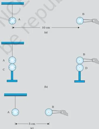
Why a coulomb is a huge unit: two charges of \( 1\ \text{C} \) placed 1 m apart in vacuum repel with a force of \( 9 \times 10^9\ \text{N} \) (NCERT, p. 7). Coulomb measured the force with a torsion balance, and could produce charges in steps of \( q/2 \) by touching a charged sphere to an identical uncharged one, the charge spreading equally (NCERT, p. 7).
The vector form keeps direction automatic:
\[ \mathbf{F}_{21} = \frac{1}{4\pi\varepsilon_0}\frac{q_1 q_2}{r_{21}^2}\hat{\mathbf{r}}_{21} \]
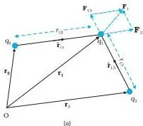
where \( \hat{\mathbf{r}}_{21} \) is the unit vector from charge 1 to charge 2. If \( q_1 q_2 \) is positive, the force is along \( \hat{\mathbf{r}}_{21} \) — repulsion; if negative, along \( -\hat{\mathbf{r}}_{21} \) — attraction. One equation handles both cases (NCERT, p. 8).
Exchanging the labels gives \( \mathbf{F}_{12} = -\mathbf{F}_{21} \), so Coulomb’s law is consistent with Newton’s third law (NCERT, p. 8). The electric force is also enormously stronger than gravity: for an electron and a proton, the ratio of electric to gravitational force is about \( 10^{39} \) (NCERT, p. 9).
Superposition: force from many charges
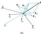
Coulomb’s law answers the two-charge problem. Superposition answers the many-charge problem: the force on any one charge is the vector sum of the forces on it due to every other charge, taken one at a time, and each individual force is unaffected by the presence of the others (NCERT, p. 11).
The addition uses the ordinary parallelogram law of vectors, and it works because each pair of charges interacts independently of the rest. The book’s summary is sweeping: all of electrostatics follows from Coulomb’s law plus superposition (NCERT, p. 12).
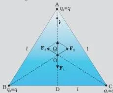
Symmetry often does the work for you. In Example 1.5, three equal charges at the vertices of an equilateral triangle all push a charge \( Q \) at the centroid with equal forces along the three medians; by symmetry these cancel exactly, and the net force on \( Q \) is zero (NCERT, p. 12-13).
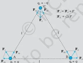
The same idea closes Example 1.6, where the vector sum of the forces on all three charges of a system is zero — a direct consequence of Newton’s third law, since every internal action has an equal and opposite reaction (NCERT, p. 13).
Electric field: the property of space around a charge
Why introduce a field when Coulomb’s law already gives the force? The chapter’s argument: when a charge \( q \) is removed, what remains at its point? A second charge placed there later still feels a force, so the influence of the original charge must exist in space itself. That influence is the electric field.
The field is defined as the force per unit positive test charge, with the test charge made vanishingly small so it does not disturb the source charge (NCERT, p. 15):
\[ \mathbf{E} = \lim_{q \to 0}\frac{\mathbf{F}}{q} \]
Its SI unit is N/C (NCERT, p. 14). The charge producing the field is the source charge; the small charge probing it is the test charge (NCERT, p. 15).
Because \( \mathbf{F} \) is proportional to \( q \), the ratio \( \mathbf{F}/q \) is independent of the test charge — the field belongs to the source charge alone. For a point charge \( Q \):
\[ \mathbf{E}(\mathbf{r}) = \frac{1}{4\pi\varepsilon_0}\frac{Q}{r^2}\hat{\mathbf{r}} \]
radially outward for \( +Q \) and radially inward for \( -Q \). Its magnitude is the same at equal distances from \( Q \) — a spherical symmetry that Gauss’s law will exploit (NCERT, p. 14-15).
For a system of charges, the field at a point is the vector sum of the fields of the individual charges, each computed as if the others were absent (NCERT, p. 15).
The field is more than a bookkeeping trick. In electrostatics it is convenient but not necessary; its real significance appears with time-dependent phenomena. The effect of a moving charge cannot travel faster than light, so the influence propagates as electromagnetic waves at speed \( c \); the field carries energy and obeys laws of its own (NCERT, p. 16).
Worked example with original numbers
Two point charges, \( +5\ \mu\text{C} \) and \( -3\ \mu\text{C} \), are 12 cm apart in air. The problem asks three things in order: the force between them, the field at the midpoint, and the force on a test charge placed there — the three ideas of Sections 1.5 to 1.7 working together.
Step 1: Convert to SI units.
\( q_1 = +5\ \mu\text{C} = +5 \times 10^{-6}\ \text{C} \), \( q_2 = -3\ \mu\text{C} = -3 \times 10^{-6}\ \text{C} \), \( r = 12\ \text{cm} = 0.12\ \text{m} \).
Step 2 (part a): Coulomb’s law uses the product of the magnitudes of the charges; the signs decide only the nature of the force.
\[ F = \frac{1}{4\pi\varepsilon_0}\frac{|q_1 q_2|}{r^2} = \frac{(9 \times 10^9)(5 \times 10^{-6})(3 \times 10^{-6})}{(0.12)^2} = \frac{0.135}{0.0144} \approx 9.4\ \text{N} \]
Part (a) answer: magnitude \( F \approx 9.4\ \text{N} \), and since the charges are unlike, the force is attractive.
Step 3 (part b): At the midpoint, each charge is \( 0.06\ \text{m} \) away.
Fix directions first: the field of \( +5\ \mu\text{C} \) points away from it, and the field of \( -3\ \mu\text{C} \) points toward it — so both point the same way, toward the negative charge, and the magnitudes add.
\[ E = \frac{(9 \times 10^9)(5 \times 10^{-6})}{(0.06)^2} + \frac{(9 \times 10^9)(3 \times 10^{-6})}{(0.06)^2} = 1.25 \times 10^7 + 7.5 \times 10^6 = 2.0 \times 10^7\ \text{N/C} \]
Part (b) answer: \( E \approx 2.0 \times 10^7\ \text{N/C} \), directed toward the \( -3\ \mu\text{C} \) charge.
Step 4 (part c): The force on a test charge is \( \mathbf{F} = q\mathbf{E} \), so only one multiplication remains.
Strictly, the field is defined with a vanishingly small test charge; the calculation here follows the book’s method of finding \( F = qE \) once \( E \) is known.
\[ F = qE = (1 \times 10^{-6})(2.0 \times 10^7) = 20\ \text{N} \]
Part (c) answer: force \( F = 20\ \text{N} \) on the \( +1\ \mu\text{C} \) test charge, in the direction of the field — pulled toward the \( -3\ \mu\text{C} \) charge.
Electric field lines
Field lines are Faraday’s pictorial map of the field, invented to visualise electric fields without heavy mathematics (NCERT, p. 20). They let you see direction and strength at a glance.
The tangent rule: at every point, the tangent to a field line gives the direction of the net field at that point, with an arrow fixing the sense (NCERT, p. 20-21).
The density rule: the relative closeness of lines shows the field’s strength — lines crowd where the field is strong and spread out where it is weak (NCERT, p. 19-20). How many lines you draw is arbitrary; only the relative density matters (NCERT, p. 19).
- Field lines start at positive charges and end at negative charges; for a single charge they start or end at infinity (NCERT, p. 21).
- In a charge-free region, field lines are continuous curves without breaks (NCERT, p. 21).
- Two field lines never cross — at a crossing, the field would not have a unique direction (NCERT, p. 21).
- Electrostatic field lines never form closed loops, because the electrostatic field is conservative — a point Chapter 2 returns to (NCERT, p. 21).
Electric dipole: moment and field
An electric dipole is a pair of equal and opposite point charges \( +q \) and \( -q \) separated by a distance \( 2a \). Its total charge is zero, yet its field is not zero — and that surprising fact drives much of the chapter’s physics (NCERT, p. 23).
The dipole moment is a vector of magnitude \( q \times 2a \), directed from the negative charge to the positive charge (NCERT, p. 24):
\[ \mathbf{p} = q \times 2a\,\hat{\mathbf{p}} \]
Students reverse this direction constantly, so fix it now: the arrow runs \( -q \to +q \).
At distances far compared with the separation (\( r \gg 2a \)), the dipole field has two simple forms. On the axis, along \( \mathbf{p} \):
\[ \mathbf{E} = \frac{2\mathbf{p}}{4\pi\varepsilon_0 r^3} \]
On the equatorial plane, opposite to \( \mathbf{p} \):
\[ \mathbf{E} = -\frac{\mathbf{p}}{4\pi\varepsilon_0 r^3} \]
Both fall off as \( 1/r^3 \), faster than the \( 1/r^2 \) of a point charge, because at large distances the fields of \( +q \) and \( -q \) nearly cancel; only the product \( qa \) survives, and that product is the dipole moment (NCERT, p. 23-24). Mnemonic: axis double, equator half, in opposite directions.
In a uniform external field, the dipole feels equal and opposite forces \( q\mathbf{E} \) and \( -q\mathbf{E} \): net force zero, but because the forces act at different points they form a couple.
The torque is \( \boldsymbol{\tau} = \mathbf{p} \times \mathbf{E} \), of magnitude \( pE\sin\theta \), and it rotates the dipole until it aligns with the field (NCERT, p. 27).
Dipoles also explain everyday observations. Water is a polar molecule — its centres of positive and negative charge do not coincide, so it has a permanent dipole moment; \( \text{CO}_2 \) and \( \text{CH}_4 \) do not.
A charged comb attracts bits of paper by polarising them: it induces a dipole moment in each piece, and the non-uniform field of the comb then pulls the induced dipole toward it (NCERT, p. 25, 27).
Electric flux and Gauss’s law
Flux measures how much of the field passes through a surface — the electrical version of measuring how much water crosses a hoop held in a stream (NCERT, p. 21). Gauss’s law then connects the flux through any closed surface to the charge inside it, and becomes the chapter’s most powerful calculating tool.
For a small area element \( \Delta S \), flux is the dot product of the field with the area vector:
\[ \Delta \phi = \mathbf{E} \cdot \Delta \mathbf{S} = E\,\Delta S \cos\theta \]
where \( \theta \) is the angle between \( \mathbf{E} \) and the area normal. Flux is a scalar with unit N C-1 m2 (NCERT, p. 22). Because a surface can be oriented two ways, a closed surface uses the convention of the outward normal for every area element (NCERT, p. 22).
Gauss’s law states that the total flux through any closed surface equals the net charge enclosed divided by \( \varepsilon_0 \):
\[ \phi = \frac{q_{\text{enclosed}}}{\varepsilon_0} \]
— independent of the size and shape of the surface (NCERT, p. 29). The proof for a point charge uses a sphere centred on the charge, where symmetry makes the field constant and normal to the surface, so \( \phi = E \times 4\pi r^2 = q/\varepsilon_0 \) (NCERT, p. 29).
The three applications all use one method: choose a Gaussian surface that matches the symmetry — a sphere for a point or spherical charge, a cylinder for a wire, a pill-box for a sheet. The results:
- Infinitely long charged wire (cylindrical surface): \( E = \dfrac{\lambda}{2\pi\varepsilon_0 r} \), radial (NCERT, p. 33).
- Infinite plane sheet (pill-box surface): \( E = \dfrac{\sigma}{2\varepsilon_0} \), perpendicular to the sheet and independent of distance from it (NCERT, p. 34).
- Spherical shell (concentric Gaussian spheres): outside, \( E = \dfrac{q}{4\pi\varepsilon_0 r^2} \) — the shell acts like a point charge at its centre; inside, \( E = 0 \), because the Gaussian sphere encloses no charge and symmetry forces the field to vanish (NCERT, p. 35).
Notice the central idea of the shell result: inside the shell the field is zero everywhere despite the shell carrying charge, because a Gaussian surface inside encloses no charge at all. The shell result is the cleanest demonstration of why Gauss’s law is a calculation tool and not just a bookkeeping identity.
Worked example: flux of a point charge through one face of a cube
A \( +2\ \mu\text{C} \) point charge sits at the centre of a cube of side 10 cm. Two questions: the total flux through the whole cube, and the flux through a single face.
Step 1: By Gauss’s law, the total flux through any closed surface depends only on the enclosed charge — not on the cube’s size or shape.
Convert \( q = +2\ \mu\text{C} = 2 \times 10^{-6}\ \text{C} \).
\[ \phi = \frac{q}{\varepsilon_0} = \frac{2 \times 10^{-6}}{8.854 \times 10^{-12}} = 2.26 \times 10^{5}\ \text{N m}^2/\text{C} \]
Step 2: The charge sits at the centre, so the six faces are identical by symmetry.
Each face catches exactly one sixth of the total flux.
\[ \phi_{\text{face}} = \frac{\phi}{6} = \frac{2.26 \times 10^5}{6} \approx 3.8 \times 10^4\ \text{N m}^2/\text{C} \]
Answers: total flux through the cube \( 2.26 \times 10^5\ \text{N m}^2/\text{C} \); flux through one face \( \approx 3.8 \times 10^4\ \text{N m}^2/\text{C} \). Notice that the 10 cm side never entered the calculation — that is Gauss’s law’s independence from surface size in action.
Formulas in This Chapter, With Symbols and Units
This is the revision-night sheet. Each formula appears with every symbol explained, its SI unit, and the situation it belongs to. Constants to keep ready: \( k = 1/(4\pi\varepsilon_0) \approx 9 \times 10^9\ \text{N m}^2/\text{C}^2 \) and \( \varepsilon_0 = 8.854 \times 10^{-12}\ \text{C}^2\ \text{N}^{-1}\ \text{m}^{-2} \).
| Formula | What each symbol means | SI unit of result | Use it when |
|---|---|---|---|
| \( q = ne \) | \( q \): charge on a body; \( n \): any integer; \( e = 1.6 \times 10^{-19}\ \text{C} \) | C | Counting charge as multiples of the basic unit (p. 5) |
| \( F = \frac{1}{4\pi\varepsilon_0}\frac{|q_1 q_2|}{r^2} \) | \( q_1, q_2 \): the two charges; \( r \): separation; \( \varepsilon_0 \): permittivity of free space | N | Magnitude of force between two point charges in vacuum (p. 6, 8) |
| \( \mathbf{F}_{21} = \frac{1}{4\pi\varepsilon_0}\frac{q_1 q_2}{r_{21}^2}\hat{\mathbf{r}}_{21} \) | \( \hat{\mathbf{r}}_{21} \): unit vector from charge 1 to charge 2; signs of the charges handled automatically | N | Force including direction — one equation for like and unlike charges (p. 8) |
| \( \mathbf{E}(\mathbf{r}) = \frac{1}{4\pi\varepsilon_0}\frac{Q}{r^2}\hat{\mathbf{r}} \) | \( Q \): source charge; \( r \): distance from it; \( \hat{\mathbf{r}} \): unit vector away from \( Q \) | N/C | Field of a single point charge (p. 14) |
| \( \mathbf{E}(\mathbf{r}) = \frac{1}{4\pi\varepsilon_0}\sum_i \frac{q_i}{r_{iP}^2}\hat{\mathbf{r}}_{iP} \) | \( q_i \): each source charge; \( r_{iP} \): distance from \( q_i \) to point P; \( \hat{\mathbf{r}}_{iP} \): unit vector from \( q_i \) to P | N/C | Field of a system of charges — vector sum (p. 15) |
| \( \Delta \phi = \mathbf{E} \cdot \Delta \mathbf{S} = E\,\Delta S\cos\theta \) | \( \theta \): angle between \( \mathbf{E} \) and the area normal; \( \Delta S \): area element | N C-1 m2 | Flux through a small area element (p. 22) |
| \( \mathbf{p} = q \times 2a\,\hat{\mathbf{p}} \) | \( 2a \): separation of the charges \( +q \) and \( -q \); direction from \( -q \) to \( +q \) | C m | Defining the dipole moment of a \( \pm q \) pair (p. 24) |
| \( \mathbf{E}_{\text{axis}} = \frac{2\mathbf{p}}{4\pi\varepsilon_0 r^3} \) | \( \mathbf{p} \): dipole moment; \( r \): distance from the dipole centre, \( r \gg a \) | N/C | Far field on the dipole axis — along \( \mathbf{p} \) (p. 24) |
| \( \mathbf{E}_{\text{equator}} = -\frac{\mathbf{p}}{4\pi\varepsilon_0 r^3} \) | same as above | N/C | Far field on the equatorial plane — opposite to \( \mathbf{p} \) (p. 24-25) |
| \( \tau = pE\sin\theta \) | \( p \): dipole moment; \( E \): uniform external field; \( \theta \): angle between them | N m | Torque on a dipole in a uniform field (p. 27) |
| \( \phi = \frac{q_{\text{enclosed}}}{\varepsilon_0} \) | \( q_{\text{enclosed}} \): net charge inside the closed surface | N m2/C | Total flux through any closed surface (p. 29) |
| \( E = \frac{\lambda}{2\pi\varepsilon_0 r} \) | \( \lambda \): linear charge density; \( r \): distance from the wire | N/C | Field of an infinitely long uniformly charged wire (p. 33) |
| \( E = \frac{\sigma}{2\varepsilon_0} \) | \( \sigma \): surface charge density | N/C | Field of a uniformly charged infinite plane sheet (p. 34) |
| \( E = \frac{q}{4\pi\varepsilon_0 r^2} \) outside; \( E = 0 \) inside | \( q \): total charge on the shell; \( R \): shell radius; \( r \): distance from the centre | N/C | Field of a uniformly charged thin spherical shell (p. 35) |
Which formula to use: a decision table
When a problem gives you a geometry, this table names the formula in one glance. The mnemonic for the two dipole results: axis double, equator half, in opposite directions.
| Situation | Formula | Direction of the field |
|---|---|---|
| Point charge \( Q \), distance \( r \) | \( E = \frac{1}{4\pi\varepsilon_0}\frac{Q}{r^2} \) | Radially outward for \( +Q \), inward for \( -Q \) |
| Dipole, point on the axis, \( r \gg 2a \) | \( E = \frac{2p}{4\pi\varepsilon_0 r^3} \) | Along \( \mathbf{p} \) |
| Dipole, point on the equatorial plane, \( r \gg 2a \) | \( E = \frac{p}{4\pi\varepsilon_0 r^3} \) | Opposite to \( \mathbf{p} \) |
| Infinite line of charge, distance \( r \) | \( E = \frac{\lambda}{2\pi\varepsilon_0 r} \) | Radially away from the wire |
| Infinite plane sheet | \( E = \frac{\sigma}{2\varepsilon_0} \) | Perpendicular to the sheet, on both sides |
| Spherical shell, outside (\( r \gt R \)) | \( E = \frac{q}{4\pi\varepsilon_0 r^2} \) | Radial, as if all charge were at the centre |
| Spherical shell, inside (\( r \lt R \)) | \( E = 0 \) | No field — the Gaussian surface encloses no charge |
Figures That Carry the Chapter
![Example 1.7 An electron falls through a distance of 1.5 cm in a uniform electric field of magnitude $2.0 \times 10^4 \text{ N C}^{-1}$ [Fig. 1.10(a)].](https://www.learncbse.net/images/electric-charges-and-fields-example-1-7-an-electron-falls-through-a-distance-of-1-5-cm-i.webp "Electric Charges and Fields Class 12: NCERT Physics Chapter 1")
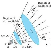
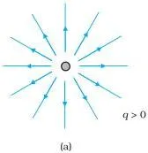
Each figure below appears in the NCERT edition with the caption given; read the caption, then the short note saying what to look for. In the printed book they appear at the page noted with each figure. Together they cover the chapter’s main visual ideas — from the first experimental rods to the Gaussian surfaces.
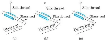
This is the experimental root of the whole chapter: two glass rods rubbed with silk repel each other, two plastic rods rubbed with fur repel each other, but a glass rod and a plastic rod attract. From experiments like these came the rule that there are exactly two kinds of charge (NCERT, p. 2).
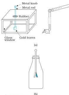
The gold-leaf electroscope is the chapter’s simple charge detector. A charged object touching the top knob sends charge down to two thin gold leaves, which diverge; the wider the spread, the greater the amount of charge (NCERT, p. 3).
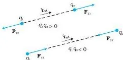
This figure keeps the vector form of Coulomb’s law straight. \( \mathbf{r}_{21} \) is the vector from charge 1 to charge 2; the force on \( q_2 \) due to \( q_1 \) acts along \( \hat{\mathbf{r}}_{21} \), and the force on \( q_1 \) due to \( q_2 \) acts in the opposite direction — Newton’s third law in action (NCERT, p. 8).
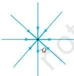
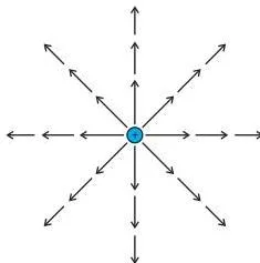
The field of a point charge is purely radial: for \( +Q \) the arrows point outward everywhere, for \( -Q \) they point inward. The magnitude is the same at equal distances from the charge — the spherical symmetry that Gauss’s law later exploits (NCERT, p. 14).
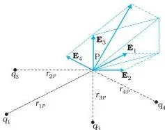
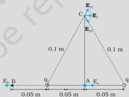
For a system of charges, the field at any point is the vector sum of the fields of the individual charges, each computed as if the others were absent. This is superposition applied to fields (NCERT, p. 15-16).
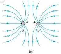
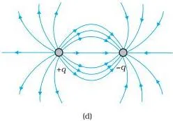
These two panels show field lines for the chapter’s basic configurations: a lone positive charge with lines radiating out, a lone negative charge with lines converging in, two like charges whose lines push apart, and a dipole whose lines curve from \( +q \) to \( -q \). From these pictures you can read off all four properties of field lines (NCERT, p. 21).
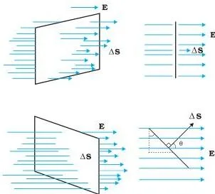
Flux depends on how the surface is held. Field lines crossing the area at \( 90^\circ \) give maximum flux; tilting the surface by an angle \( \theta \) reduces it to \( E\,\Delta S\cos\theta \), and at \( 90^\circ \) the lines run along the surface and no flux crosses at all (NCERT, p. 22).
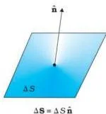
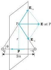
The dipole field on the axis points along \( \mathbf{p} \), while on the equatorial plane it points exactly opposite to \( \mathbf{p} \). Notice that \( \mathbf{p} \) itself is drawn from the negative to the positive charge — reversing it is the classic mistake (NCERT, p. 24).
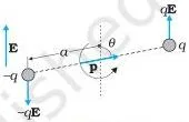
A dipole in a uniform field feels equal and opposite forces \( q\mathbf{E} \) and \( -q\mathbf{E} \). Because the forces act at different points, they form a couple: no net force, but a torque that rotates the dipole until it aligns with the field (NCERT, p. 27).
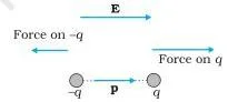
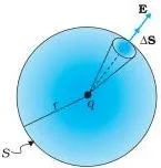
This sphere is the Gaussian surface that proves Gauss’s law for a point charge. By symmetry the field is perpendicular to the sphere and has the same magnitude everywhere on it, so \( \phi = E \times 4\pi r^2 = q/\varepsilon_0 \) (NCERT, p. 29).
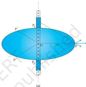
For an infinitely long wire the field is radial, so the natural Gaussian surface is a cylinder centred on the wire. Field lines cross only the curved wall, giving \( E = \lambda/(2\pi\varepsilon_0 r) \) (NCERT, p. 33).
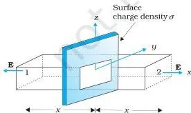
For an infinite sheet the natural Gaussian surface is a pill-box straddling the sheet. Field lines leave both flat faces; because the flux divides between two faces, the result is \( E = \sigma/(2\varepsilon_0) \), independent of distance from the sheet (NCERT, p. 34).
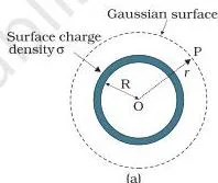
Two concentric Gaussian spheres around a charged spherical shell: outside (\( r \gt R \)) the shell behaves as a point charge, \( E = q/(4\pi\varepsilon_0 r^2) \); inside (\( r \lt R \)) the Gaussian sphere encloses no charge, so \( E = 0 \) (NCERT, p. 35).
Definitions You Should Know
These are the formal terms of the chapter, in the order the book introduces them. Each definition is one plain sentence you can reproduce, with the page where the book defines it.
| Term | Definition |
|---|---|
| Electric charge / electrification | The property that makes a body attract or repel other charged bodies; an object that possesses it is said to be electrified or charged (p. 2). |
| Point charge | A charged body whose size is very small compared with the distances involved, so all its charge is treated as concentrated at one point (p. 4). |
| Conductor | A substance that readily allows electricity to pass through it because its electrons are comparatively free to move (p. 3). |
| Insulator | A substance that offers high resistance to the passage of electricity, so charge stays where it is placed (p. 3). |
| Quantisation of charge | The fact that all free charges are integral multiples of the basic unit \( e \) — charge can only change in steps of \( e \) (p. 5). |
| Coulomb (C) | The SI unit of charge, defined through electric current; one coulomb is the charge flowing in one second when the current is one ampere (p. 5). |
| Permittivity of free space (\( \varepsilon_0 \)) | The constant in Coulomb’s law, \( \varepsilon_0 = 8.854 \times 10^{-12}\ \text{C}^2\ \text{N}^{-1}\ \text{m}^{-2} \), relating force, charges and distance in vacuum (p. 8). |
| Source charge | The charge that produces the electric field being studied (p. 15). |
| Test charge | A charge so small that it does not disturb the source charge, used to probe the field (p. 15). |
| Electric field | The force per unit positive test charge at a point, \( \mathbf{E} = \mathbf{F}/q \) in the limit \( q \to 0 \); unit N/C (p. 14). |
| Electric field line | A curve whose tangent at every point gives the direction of the net field there, with an arrow showing the sense (p. 20-21). |
| Electric flux | The scalar \( \mathbf{E} \cdot \Delta \mathbf{S} = E\,\Delta S\cos\theta \), proportional to the number of field lines crossing the area element; unit N C-1 m2 (p. 22). |
| Electric dipole | A pair of equal and opposite point charges \( +q \) and \( -q \) separated by a distance \( 2a \) (p. 23). |
| Dipole moment | The vector \( \mathbf{p} = q \times 2a\,\hat{\mathbf{p}} \) of magnitude charge times separation, directed from \( -q \) to \( +q \); unit C m (p. 24). |
| Linear / surface / volume charge density (\( \lambda, \sigma, \rho \)) | Charge per unit length, per unit area and per unit volume, used when charge is spread continuously along a line, over a surface or through a volume (p. 28). |
| Gaussian surface | A closed surface chosen so that the field has constant magnitude (or is zero) over parts of it, making Gauss’s law a practical way to find \( E \) (p. 32-33). |
Common Mistakes Students Make in This Chapter
The mistakes below are the ones this chapter invites, and each correction is grounded in the chapter text. Read them before you start solving, not after.
| Mistake | Correct rule | How to check your answer |
|---|---|---|
| Adding charges inside Coulomb’s law | The law uses the product of the magnitudes \( |q_1 q_2| \); signs only decide attraction or repulsion (p. 6-8). | Compute the force with magnitudes only — it must come out positive; then attach “attractive” or “repulsive” from the signs. |
| Pointing the dipole moment from \( +q \) to \( -q \) | The dipole moment runs from \( -q \) to \( +q \) (p. 23-24). | Sketch the charges and draw the arrow from the negative charge to the positive one before substituting numbers. |
| Treating field lines as paths a charge follows | The tangent at a point gives the force direction on a unit positive charge placed there; the line is not a trajectory (p. 20). | Ask “force at this point on a +1 C charge?” and use the tangent, not the whole curve. |
| Drawing two field lines that cross | Two field lines never cross — the field would not have a unique direction at the crossing (p. 21). | At every crossing there must be a single tangent; if two tangents appear, the picture is wrong. |
| Calling electric flux a vector | Flux is the scalar \( E\,\Delta S\cos\theta \), a dot product (p. 22). | Check the unit: N C-1 m2, not N/C. |
| Expecting flux to change when a closed surface is reshaped or resized | For a closed surface, flux depends only on the enclosed charge: \( \phi = q/\varepsilon_0 \) (p. 29-30). | Ask whether the new surface still encloses the same charge; if it does, the flux is unchanged. |
| Using Gauss’s law on any surface and reading off \( E \) | The law is always true, but \( E \) comes out of the integral only when symmetry makes it constant on the surface (p. 32). | Choose the Gaussian surface first and argue why \( E \) is constant on it before writing \( \phi = E \times \text{area} \). |
| Assuming charge inside a surface means the field is non-zero everywhere on it | Gauss’s law gives total flux, not the local field; the local field needs symmetry to be deducible (p. 32-35). | Recall the shell: the field inside is zero although the shell itself carries charge. |
Exam Notes: How the Exercises Test These Ideas
The exercise set at the end of the chapter is arranged almost like a syllabus: each idea appears once, roughly in the order the chapter developed it. The table below pairs every exercise with the concept it tests, so revision can be targeted instead of random.
| Exercise | Concept tested |
|---|---|
| 1.1-1.3 | Coulomb’s law: force between small charged spheres, finding distance from a known force, and the dimensionless ratio \( ke^2/Gm_em_p \) comparing electric and gravitational forces |
| 1.4-1.5 | Quantisation and conservation of charge as concept questions |
| 1.6 and 1.12 | Superposition with symmetry (four charges at the corners of a square) and Coulomb’s law under doubling and halving |
| 1.7 | Properties of field lines: why they are continuous and why they never cross |
| 1.8 | Electric field of two equal-and-opposite charges at the midpoint, plus the force on a test charge placed there |
| 1.9 | Total charge and electric dipole moment of a two-charge system (the net charge of a dipole is zero) |
| 1.10 | Torque on a dipole in a uniform field, \( \tau = pE\sin\theta \) |
| 1.11 | Quantisation in use: counting the electrons transferred and the mass transferred with them |
| 1.13 | Reading charge signs and charge-to-mass ratio from field-line tracks (Fig. 1.30) |
| 1.14-1.15 | Electric flux through a square (\( E\,\Delta S\cos\theta \) with orientation) and net flux through a cube in a uniform field (zero, since no charge is enclosed) |
| 1.16-1.19 | Gauss’s law: enclosed charge from measured flux, flux through one face of a cube, and flux unchanged when the Gaussian radius doubles |
| 1.20-1.21 | Conducting sphere: field outside, net charge, total flux and surface charge density |
| 1.22 | Infinite line charge: linear charge density from the field it produces |
| 1.23 | Parallel plates: field in the outer regions (zero) and between the plates (\( \sigma/\varepsilon_0 \)) |
The exercise set produces three kinds of work:
- Direct numericals — computing force, field, torque or flux from given charges and distances (Exercises 1.1, 1.2, 1.8, 1.10, 1.12, 1.14, 1.18, 1.20-1.23).
- Applications of derived results — the dipole far-field formulas (Section 1.10) and the three Gauss’s-law results (Section 1.14) are derived in the text, and Exercises 1.9, 1.10 and 1.16-1.23 expect you to apply them.
- Concept and property questions — quantisation, conservation, field-line properties and flux through closed surfaces (Exercises 1.4, 1.5, 1.7, 1.9, 1.15, 1.16, 1.19).
Textbook contents and the examinable syllabus are not always identical. Before planning revision for a board year, check the current official CBSE syllabus to confirm exactly which parts of this chapter it lists. NCERT settles the book; CBSE settles what is examined from it.
Revision Summary: The Chapter as a Checklist
The checklist below follows the chapter’s own closing SUMMARY and POINTS TO PONDER, in the order the ideas build. If you can say each line without looking, the chapter is done.
- Two kinds of charge; like repel, unlike attract; bodies get charged by gaining or losing electrons.
- Three basic properties: additivity (charges add as signed scalars), conservation (isolated systems), quantisation (\( q = ne \)).
- Coulomb’s law: \( F = \frac{1}{4\pi\varepsilon_0}\frac{|q_1 q_2|}{r^2} \), with \( k \approx 9 \times 10^9\ \text{N m}^2/\text{C}^2 \); the vector form carries the direction.
- Superposition: the force on any charge is the vector sum of the pairwise forces.
- Electric field: \( \mathbf{E} = \mathbf{F}/q \) with \( q \to 0 \); a point charge gives \( \mathbf{E} = \frac{1}{4\pi\varepsilon_0}\frac{Q}{r^2}\hat{\mathbf{r}} \); a system’s field is a vector sum.
- Field lines: tangent gives direction, density gives strength; four properties — start at \( + \), end at \( – \), continuous in charge-free regions, never cross, never form closed loops.
- Electric flux: \( \Delta\phi = E\,\Delta S\cos\theta \), unit N C-1 m2.
- Dipole: \( \mathbf{p} = q \times 2a\,\hat{\mathbf{p}} \) from \( -q \) to \( +q \); axis field \( \frac{2\mathbf{p}}{4\pi\varepsilon_0 r^3} \), equatorial field \( -\frac{\mathbf{p}}{4\pi\varepsilon_0 r^3} \).
- Torque in a uniform field: \( \tau = \mathbf{p} \times \mathbf{E} \), magnitude \( pE\sin\theta \), aligning the dipole.
- Gauss’s law: \( \phi = q_{\text{enclosed}}/\varepsilon_0 \) through any closed surface.
- Three applications: infinite wire \( E = \frac{\lambda}{2\pi\varepsilon_0 r} \); infinite sheet \( E = \frac{\sigma}{2\varepsilon_0} \); spherical shell \( E = \frac{q}{4\pi\varepsilon_0 r^2} \) outside and \( E = 0 \) inside.
Related Resources
This listing is maintained for the 2026-27 academic session using the NCERT textbook information available to us. NCERT remains the authority for confirming the latest edition.
This chapter is the opening of electrostatics; the next chapter builds directly on it, so it is the natural next stop when you finish here.
- NCERT Class 12 Physics book page — every chapter of Physics Part I and Part II, with its own PDF and walkthrough
- Next chapter: Electrostatic Potential and Capacitance — the chapter that takes Coulomb’s law and the field into work and potential
- Class 12 books hub — all Class 12 NCERT books indexed in one place
- Class 12 Physics revision notes — revision-focused treatment of this chapter’s ideas
- Class 12 revision hub — notes across all Class 12 subjects
- CBSE notes index — notes across all classes and subjects
- Electrostatic Potential and Capacitance revision notes — the next chapter’s ideas in notes form
Sources and Data Verification
- This page describes the NCERT Class 12 Physics Part I textbook, Chapter 1, Electric Charges and Fields — the official NCERT edition published on ncert.nic.in. All section headings, figure captions and page numbers on this page come from that edition.
- It covers Chapter 1 of Physics Part I. It does not cover Physics Part II, other Class 12 subjects, or books from other streams.
- This listing is maintained for the current CBSE academic session.
- NCERT settles textbooks, editions and the official PDFs; CBSE settles the curriculum, syllabus and examinations. As with every chapter, textbook contents and the examinable syllabus are not always identical — check the current official CBSE syllabus before planning revision.
Frequently Asked Questions
Why is the electric field inside a uniformly charged spherical shell zero?
Because a Gaussian sphere drawn inside the shell encloses no charge. By Gauss’s law its flux is zero, and by spherical symmetry the field must be constant and normal to that sphere — so the field itself is zero everywhere inside (NCERT, p. 35).
Why can two electric field lines never cross?
If two lines crossed, the field would have two different directions at the same point. But the field has one unique direction at every point, so a crossing is impossible (NCERT, p. 21).
How many electrons make one coulomb of charge?
About \( 6 \times 10^{18} \). One electron carries \( e = 1.6 \times 10^{-19}\ \text{C} \), so dividing 1 C by \( e \) gives roughly \( 6 \times 10^{18} \) electrons (NCERT, p. 5).
Why does the electric field of a dipole fall off as \( 1/r^3 \) and not \( 1/r^2 \)?
Because at large distances the fields of \( +q \) and \( -q \) almost cancel. The cancellation removes the \( 1/r^2 \) term, and what remains falls off as \( 1/r^3 \), depending on the product \( q \times 2a \) — the dipole moment — rather than on \( q \) and \( a \) separately (NCERT, p. 23-24).
Does the electric flux through a closed surface depend on the size or shape of the surface?
No. For any closed surface, the total flux equals the enclosed charge divided by \( \varepsilon_0 \), independent of the size and shape of the surface (NCERT, p. 29). Reshaping the surface changes where the field crosses it, not the total count of field lines crossing it.
Why do we ignore quantisation of charge for macroscopic bodies?
Because the basic unit \( e \) is unimaginably small compared with macroscopic charges. A charge of just \( 1\ \mu\text{C} \) already contains about \( 10^{13} \) electronic charges, so changing in steps of \( e \) is invisible — like a dotted line that looks continuous from a distance (NCERT, p. 5-6).
Reference: NCERT Class 12 Physics Part I textbook, chapter 1, official edition on ncert.nic.in.
Explore Class 12 Physics Books
Class 12 Physics on LearnCBSE:
Related chapters: