
Looking for Chapter Three Current Electricity Class 12? This page gives you the official NCERT PDF of Chapter 3 Current Electricity from Physics Part I — the chapter runs across printed pages 80 to 106 — along with a section-by-section walkthrough of what it teaches, so you know exactly what is in the file before you open it.
Download the NCERT Class 12 Physics Chapter 3 Current Electricity PDF
The official NCERT file for this chapter of Physics Part I — printed pages 80 to 106 of the current edition — is the NCERT Class 12 Physics Chapter 3 Current Electricity PDF: open it for the full text, every figure and the complete set of exercises in the original book layout. The same file is indexed as leph103.pdf on ncert.nic.in.
| What the chapter holds | Count | Where it is used |
|---|---|---|
| Printed pages | 26 | |
| Sections in the chapter | 14 | |
| Figures with NCERT captions | 20 | |
| Tables | 1 | |
| Worked examples | 1 | solved step by step in our NCERT Solutions |
| Exercise questions | 9 | answered in our NCERT Solutions |
| Official NCERT PDF | Download the chapter PDF | the chapter exactly as NCERT publishes it |
Chapter Three Current Electricity Class 12 at a Glance
The table below shows how much the chapter holds — its sections, figures, worked examples and exercise questions — so you can judge the file’s size at a glance. The walkthrough that follows says what each piece actually teaches.
What this chapter covers
This roadmap names every section of the chapter with its printed page, phrased as the question each section answers. It is a map, not a summary — the summaries come further down.
- 3.1 Introduction (p. 81) — flips from charges at rest in Chapter 1 to charges in motion: lightning as a violent unsteady current, a torch and a cell-driven clock as steady ones.
- 3.2 Electric current (p. 81) — defines current as the net charge crossing an area per unit time, and introduces the ampere.
- 3.3 Electric currents in conductors (p. 82) — why free electrons alone give no current, and why a steady current needs a source that keeps the field alive.
- 3.4 Ohm’s law (p. 83) — \(V \propto I\), and the slab argument that locates resistance in length and cross-section: \(R = \rho l/A\).
- 3.5 Drift of electrons and the origin of resistivity (p. 85) — asks the question everyone asks: if electrons drift at about a millimetre per second, why does the bulb light instantly?
- 3.5.1 Mobility (p. 88) — compares how freely different charge carriers move per unit field.
- 3.6 Limitations of Ohm’s law (p. 89) — the three ways a device can break the \(V\)–\(I\) proportionality.
- 3.7 Resistivity of various materials (p. 89) — where metals, semiconductors and insulators sit on the resistivity scale.
- 3.8 Temperature dependence of resistivity (p. 90) — why metals resist more when hot, but semiconductors resist less.
- 3.9 Electrical energy, power (p. 92) — \(P = IV\), the heat a conductor dissipates, and why transmission lines carry enormous voltages.
- 3.10 Cells, emf, internal resistance (p. 93) — what emf really is, and why a cell’s terminal voltage drops when current flows.
- 3.11 Cells in series and in parallel (p. 95) — replacing stacks of cells by one equivalent cell.
- 3.12 Kirchhoff’s rules (p. 97) — the junction and loop rules that solve any network, however tangled.
- 3.13 Wheatstone bridge (p. 100) — a four-arm resistance network that homes in on an unknown resistance through a null deflection.
The chapter ends with the book’s own SUMMARY (pp. 102–104), its POINTS TO PONDER clarifications (pp. 104–105) and the end-of-chapter exercises (p. 105 onwards). The mistake list and recap on this page are built from those closing sections.
The core ideas, section by section
Each idea below opens with one or two plain sentences — what it is and why the chapter bothers with it — before any formula. Page numbers let you follow along with your own book.
What an electric current actually is
An electric current is a measured flow of charge, but the chapter is careful about how it is measured: across an area, not along a wire, because positive and negative charges can both be moving. That care is what makes the definition exact.
For a steady flow, current is the net charge crossing an area in time \(t\), \(I = q/t\). More generally, the current at an instant is the limit of that ratio as the time interval shrinks:
\[ I(t) = \lim_{\Delta t \to 0} \frac{\Delta Q}{\Delta t} \]
The bookkeeping uses \(q = q_+ – q_-\): the net amount of positive charge moving with the flow, minus the net amount moving against it. If the answer comes out negative, the net current is in the backward direction (NCERT, p. 82).
The SI unit is the ampere (A). The chapter’s own scale: domestic appliances draw currents of the order of amperes, lightning carries tens of thousands of amperes, and currents in our nerves are in microamperes (NCERT, p. 82). One point worth fixing now: current is a scalar.
The chapter proves it later through \(I = \mathbf{j} \cdot \Delta \mathbf{S}\), a dot product of two vectors, and currents at a junction add arithmetically, never as vectors (NCERT, p. 104).
Why a steady current needs a source
In a metal, electrons are free to move — so why is there no current without a battery? Because thermal motion is random. An electron collides with a fixed ion, bounces off with the same speed in a random direction, and repeats.
At any instant, as many electrons travel one way as the opposite way, the average velocity is zero, and there is no net current (NCERT, p. 82).

The cylinder in Fig. 3.1 shows what it takes to get a net flow. Putting \( +Q \) on one end and \( -Q \) on the other creates a field; electrons drift and neutralise the charges, and the current stops after a short while.
A cell or battery continuously replenishes the ends, keeping the field steady — that is the job of every source in this chapter (NCERT, p. 83). In solid conductors only electrons carry the current; in electrolytic solutions, positive and negative ions both move (NCERT, p. 82).
Ohm’s law and where resistance comes from
Ohm’s law is the empirical result, found in 1828, that for many conductors the current is proportional to the voltage across them. Written as \(V = RI\), it names the constant \(R\) the resistance, with the unit ohm (\(\Omega = \text{V/A}\)). Resistance depends on material, length and area — and Fig. 3.2 shows exactly how the geometry enters.

Two identical slabs placed end to end carry the same current as one slab, but the voltage doubles, so the resistance doubles: \(R \propto l\). Cutting the same slab lengthwise gives each half the same voltage but half the current, so each half has double the resistance: \(R \propto 1/A\). Together they give \[ R = \rho \frac{l}{A} \]
where \(\rho\) is the resistivity — a property of the material, not of the dimensions (NCERT, p. 84). Dividing by area also defines the current density \(j = I/A\), in A/m², and Ohm’s law takes the local form \(E = j\rho\), or in vector form \(\mathbf{j} = \sigma \mathbf{E}\), with \(\sigma = 1/\rho\) the conductivity (NCERT, p. 85).
Worked check with original numbers: a wire is 8.0 m long, has cross-section \(3.0 \times 10^{-6}\ \text{m}^2\), and its measured resistance is \(0.12\ \Omega\).
Step 1: Rearrange \(R = \rho l / A\) for resistivity: \(\rho = RA/l\).
\[ \rho = \frac{0.12 \times 3.0 \times 10^{-6}}{8.0} = 4.5 \times 10^{-8}\ \Omega\, \text{m} \]
Final answer: \(\rho = 4.5 \times 10^{-8}\ \Omega\, \text{m}\) — the right order for a good metal like copper, and the unit is ohm-metre (\(\Omega\, \text{m}\)).
Drift velocity: the microscopic origin of Ohm’s law
Here is the surprise of the chapter: the field accelerates electrons, yet their average velocity is steady. Collisions explain it, and the three steps below are the whole argument (NCERT, pp. 85–87).
- Random after every collision. The velocity an electron brings out of a collision has no preferred direction, so averaged over all electrons it contributes zero.
- The field adds one small term. Between collisions an electron accelerates for an average time \(\tau\), the relaxation time. The average velocity becomes \(\mathbf{v}_d = -e\mathbf{E}\tau/m\) — the drift velocity, independent of time. The minus sign means electrons drift opposite the field.
- Turn drift into current. The cylinder argument of Fig. 3.4 gives \(I = neAv_d\), and comparing with \(\mathbf{j} = \sigma \mathbf{E}\) identifies the conductivity \(\sigma = ne^2\tau/m\). That is Ohm’s law emerging from a microscopic picture.
The book’s Example 3.1 computes a real number: conduction electrons in a copper wire carrying 1.5 A drift at about 1.1 mm/s (NCERT, p. 87). Here is a second one with fresh values.
- Step 1: Note the data: \(A = 2.0 \times 10^{-6}\ \text{m}^2\), \(I = 5.0\ \text{A}\), \(n = 8.5 \times 10^{28}\ \text{m}^{-3}\), \(e = 1.6 \times 10^{-19}\ \text{C}\).
- Step 2: Apply \(v_d = I/(neA)\), the same formula the book uses in Example 3.1.
\[ v_d = \frac{5.0}{8.5 \times 10^{28} \times 1.6 \times 10^{-19} \times 2.0 \times 10^{-6}} = 1.8 \times 10^{-4}\ \text{m/s} \]
Final answer: \(v_d \approx 1.8 \times 10^{-4}\ \text{m/s}\) (about 0.2 mm/s) — roughly a million times smaller than the thermal speeds of the atoms, and over a trillion times smaller than the speed at which the field itself propagates along the conductor (NCERT, p. 87).
Both drift diagrams (Figs. 3.3 and 3.4) are unpacked in the figure walkthrough below.
Mobility: comparing how freely charge carriers move
Mobility asks a fair comparison question: given the same field, which carriers move fastest? It is the drift speed per unit field, \[ \mu = \frac{|v_d|}{E} = \frac{e\tau}{m} \]
always positive, with SI unit \( \text{m}^2/\text{Vs} \) (NCERT, p. 88). Wherever conductivity appears, mobile carriers sit behind it: electrons in metals, electrons plus positive ions in an ionised gas, and both positive and negative ions in an electrolyte (NCERT, p. 88). The quantity to remember is the ratio itself, not the drift speed alone.
When Ohm’s law fails
Ohm’s law holds for a large class of materials, but it is not a fundamental law of nature. The chapter lists three distinct ways a device can depart from it (NCERT, p. 89).
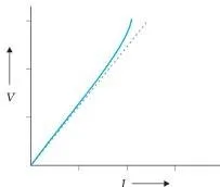
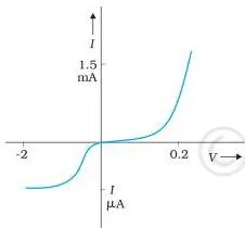
Figure 3.5 is the first failure: at high currents a real conductor’s \(V\)–\(I\) curve bends away from the dashed straight line. The second failure, in Fig. 3.6, is sign dependence: a diode conducts readily in one direction and almost not at all in the other, so its curve uses different scales for positive and negative voltages.
The third failure is a non-unique \(V\)–\(I\) relation: for one current there is more than one voltage, as in gallium arsenide, GaAs (mentioned in the text; its Fig. 3.7 is not reproduced here). Non-ohmic devices are everywhere in electronics — the chapter simply chooses to study the ohmic ones.
Resistivity and temperature: metals vs semiconductors
Resistivity changes with temperature, and it changes in opposite directions for metals and semiconductors. Over a limited range, the relation is linear:
\[ \rho_T = \rho_0 \left[ 1 + \alpha (T – T_0) \right] \]
where \(\alpha\) is the temperature coefficient of resistivity, positive for metals, with unit \((^{\circ}\text{C})^{-1}\) (NCERT, p. 90).
The microscopic formula \(\rho = m/(ne^2\tau)\) explains the direction of the effect: in a metal, heating makes collisions more frequent so \(\tau\) shrinks while \(n\) stays put — resistivity rises; in a semiconductor, heating releases so many extra carriers that \(n\) surges and resistivity falls (NCERT, p. 91).
| Material class | Typical resistivity | When heated |
|---|---|---|
| Metals | \(10^{-8}\) to \(10^{-6}\ \Omega\, \text{m}\) | Rises almost linearly over a limited temperature range |
| Semiconductors | Between metals and insulators | Falls — carrier number rises faster than \(\tau\) falls |
| Insulators (ceramic, rubber, plastics) | About \(10^{18}\) times metals or more | \(n\) rises with temperature, so resistivity falls |
Because the alloy nichrome — and manganin and constantan — show an almost flat \(\rho\)–\(T\) curve, they are used for wire-wound standard resistors whose resistance barely changes with temperature (NCERT, p. 90).
Worked check: an element has resistance 100 Ω at 27 °C and 115 Ω at its working temperature, with \(\alpha = 1.0 \times 10^{-3}\ {}^{\circ}\text{C}^{-1}\).
- Step 1: Use the same relation in resistance form: \(R_T = R_1[1 + \alpha(T_2 – T_1)]\).
- Step 2: Solve for \(T_2 – T_1 = (R_T/R_1 – 1)/\alpha\).
\[ T_2 – T_1 = \frac{115/100 – 1}{1.0 \times 10^{-3}} = 150\ {}^{\circ}\text{C} \]
Final answer: \(T_2 = 27 + 150 = 177\ {}^{\circ}\text{C}\). The book’s own Examples 3.3 and 3.4 follow this exact pattern: a toaster element settling at 847 °C and a platinum-resistance thermometer reading a bath at 345.65 °C (NCERT, pp. 91–92).
Electrical energy, power and high voltage transmission
Collisions turn the kinetic energy the field gives electrons into vibration of the atoms — that is why conductors heat. The power dissipated as heat is \[ P = IV = I^2R = \frac{V^2}{R} \]
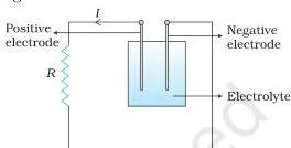
(NCERT, pp. 92–93). The energy does not appear from nowhere: in the simple circuit of Fig. 3.11, the chemical energy of the cell is the source.
The genuinely important application is transmission. For a delivered power \(P\) through cables of resistance \(R_c\), the wasted power in the cables is \[ P_c = I^2 R_c = \frac{P^2 R_c}{V^2} \]
What this says in words: for a fixed delivered power, the cable loss is inversely proportional to the square of the voltage. Double the voltage, the current halves, and since loss scales with \(I^2\), it drops to one quarter.
That is why power stations send electricity over hundreds of miles at enormous voltages, and a transformer steps the voltage down before it reaches homes and factories (NCERT, p. 93).
Cells, emf and internal resistance
emf (electromotive force) is a historical name for something that is not a force at all: a potential difference. Inside a cell, the two electrodes develop contact potential differences \(V_+\) and \(V_-\), and \[ \varepsilon = V_+ + V_- \]
When no current flows, this is exactly the voltage across the terminals — so the electromotive force (emf) is the open-circuit terminal voltage, measured in volts (NCERT, p. 94).

With a load connected, the current must push through the electrolyte itself, whose finite resistance \(r\) is the internal resistance. The terminal voltage drops (NCERT, p. 94):
\[ V = \varepsilon – Ir \]
and the current delivered to an external resistance \(R\) is \[ I = \frac{\varepsilon}{R + r} \]
Short the cell (\(R = 0\)) and \(I_{\max} = \varepsilon/r\) — but most cells would be permanently damaged long before, so the theoretical maximum is far above the safe current (NCERT, p. 95).
- Step 1: A cell has \(\varepsilon = 6.0\ \text{V}\), \(r = 0.5\ \Omega\), driving \(R = 2.5\ \Omega\).
- Step 2: Current: \(I = \varepsilon/(R + r)\).
\[ I = \frac{6.0}{2.5 + 0.5} = 2.0\ \text{A} \]
Step 3: Terminal voltage: \(V = \varepsilon – Ir\).
\[ V = 6.0 – 2.0 \times 0.5 = 5.0\ \text{V} \]
Final answer: \(I = 2.0\ \text{A}\) and terminal voltage \(V = 5.0\ \text{V}\). Note \(I_{\max} = 6.0/0.5 = 12\ \text{A}\) — six times the load current, and far more than this cell could safely supply.
Cells in series and in parallel
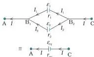
Just as resistors combine, so do cells, and a combination acts like a single equivalent cell. For two cells in series, \[ \varepsilon_{eq} = \varepsilon_1 + \varepsilon_2, \qquad r_{eq} = r_1 + r_2 \]
when the current leaves each cell from its positive electrode (NCERT, p. 95). If one cell is reversed — the current leaves it from the negative electrode — its emf enters with a minus sign: \(\varepsilon_{eq} = \varepsilon_1 – \varepsilon_2\) (NCERT, p. 96).

For cells in parallel, the internal resistances again combine like resistors, but emfs do not simply add:
\[ \frac{1}{r_{eq}} = \frac{1}{r_1} + \frac{1}{r_2}, \qquad \frac{\varepsilon_{eq}}{r_{eq}} = \frac{\varepsilon_1}{r_1} + \frac{\varepsilon_2}{r_2} \]
(NCERT, p. 96). Reversing the second cell in parallel flips \(\varepsilon_2 \to -\varepsilon_2\) in that formula. Read the pattern once and keep it: internal resistances add like resistors; emfs add only when the cells are aligned.
Kirchhoff’s rules without sign errors
Series and parallel formulas cannot crack every network. Two rules can (NCERT, p. 97):
- Junction rule — at any junction, the sum of currents entering equals the sum of currents leaving. It is conservation of charge, because steady current cannot pile charge anywhere.
- Loop rule — around any closed loop, the algebraic sum of changes in potential is zero. It is the statement that potential has one definite value at each point: come back to where you started and the net change is zero.
The skill to carry into the exam is a repeatable sign convention, so that a negative answer means something rather than causing panic.
Step 1 — label.
Draw an arrow for every branch current.
Left loop: current \(I_1\) clockwise through a 12 V battery and a 4 Ω resistor.
Right loop: current \(I_2\) clockwise through a 6 V battery (drawn opposing) and a 2 Ω resistor.
The shared branch between the loops carries \(I_1 – I_2\).
Step 2 — fix the signs.
Moving with a current through a resistor is a drop (\(-IR\)); against it is a rise (\(+IR\)).
Crossing a battery from − to + is a rise (\(+\varepsilon\)); from + to − is a drop (\(-\varepsilon\)).
Apply this to both loops.
Step 3 — write the loops.
Left loop: \(12 – 4I_1 – 2(I_1 – I_2) = 0\), which simplifies to \(3I_1 – I_2 = 6\).
Right loop: \(-2I_2 – 6 + 2(I_1 – I_2) = 0\), which simplifies to \(I_1 – 2I_2 = 3\).
Step 4 — solve.
From the first, \(I_2 = 3I_1 – 6\).
Substitute into the second: \(I_1 – 2(3I_1 – 6) = 3\), giving \(I_1 = 1.8\ \text{A}\), then \(I_2 = -0.6\ \text{A}\).
Final answer: \(I_1 = 1.8\ \text{A}\); \(I_2 = -0.6\ \text{A}\) means the true current in the right loop flows opposite to the drawn arrow — the 6 V battery is being overdriven, so it acts as a load. The shared branch carries \(I_1 – I_2 = 2.4\ \text{A}\) downward.
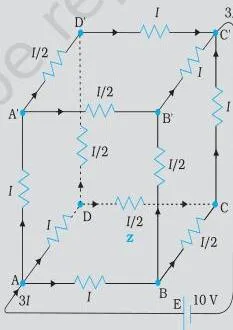
Fig. 3.16 is the book’s showcase: a cube of twelve 1 Ω resistors across a 10 V battery. Symmetry lets Kirchhoff’s rules do the work in a few lines — currents split equally at symmetric corners — giving an equivalent resistance of \(5/6\ \Omega\) and a total current of 12 A (Example 3.5, NCERT, p. 98).
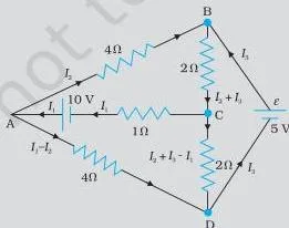
Fig. 3.17 is the general case, Example 3.6: no symmetry, three unknown branch currents \(I_1\), \(I_2\), \(I_3\), and three simultaneous equations to solve (NCERT, p. 99).
The Wheatstone bridge and the balance condition
The bridge exists to measure an unknown resistance precisely. Four resistors form a ring; a battery connects across one opposite pair (AC, the battery arm) and a galvanometer across the other (BD, the galvanometer arm). The trick: adjust until no current flows through the galvanometer, and the balance condition hands you the unknown (NCERT, p. 100).
At balance \(I_g = 0\), so the junction rule at B and D forces \(I_1 = I_3\) and \(I_2 = I_4\). Applying the loop rule to the two galvanometer loops gives the balance condition (NCERT, p. 101):
\[ \frac{R_2}{R_1} = \frac{R_4}{R_3} \]
Memory aid: at balance, the cross product of opposite arms is equal — \(R_1 R_4 = R_2 R_3\) — so the unknown is \(R_4 = R_3 \cdot R_2 / R_1\). Put the unknown in the fourth arm, keep \(R_1\) and \(R_2\) fixed, vary \(R_3\) until the galvanometer reads null, and the formula gives \(R_4\).
The meter bridge is the practical device built on this principle (NCERT, p. 101).
- Step 1: Use the balance condition \(R_4 = R_3 \cdot R_2 / R_1\).
- Step 2: Substitute \(R_1 = 20\ \Omega\), \(R_2 = 30\ \Omega\), \(R_3 = 45\ \Omega\):
\[ R_4 = 45 \times \frac{30}{20} = 67.5\ \Omega \]
Final answer: \(R_4 = 67.5\ \Omega\).
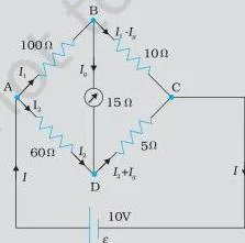
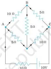
Fig. 3.19 carries Example 3.7’s own values: AB = 100 Ω, BC = 10 Ω, CD = 5 Ω, DA = 60 Ω, a 15 Ω galvanometer across BD and 10 V across AC. Read it the way the example does — label currents \(I_1\), \(I_2\) and the galvanometer current \(I_g\), then write the three meshes. The answer, 4.87 mA through the galvanometer, shows this bridge is not balanced (NCERT, p. 101).
Reading the figures that matter
These are the diagrams students misread most. Each carries a single idea; here is what to look at.
Fig. 3.3 — one electron’s zigzag path (p. 85)
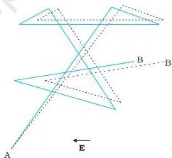
The full lines are straight-flight segments between collisions. Switch on a field and every segment bends slightly in the same direction, so the electron ends at B′ instead of B — a net drift opposite the field, tiny per collision but identical for the enormous density of free electrons per cubic metre. That is the current.
Fig. 3.4 — the cylinder that explains the current formula (p. 86)
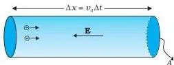
In one second, every electron within a distance \(v_d\) of the area crosses it. The cylinder of unit area and length \(v_d\) therefore contains exactly the charge that crosses per second — the geometric heart of \(I = neAv_d\). If the formula ever feels abstract, come back to this picture.
Figs. 3.8, 3.9, 3.10 — three temperature graphs, one story (p. 90)
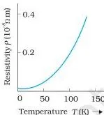
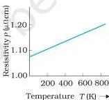
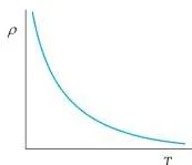
Read them as a trio. Copper’s graph climbs with a strong, nearly constant slope — the linear range where \(\alpha\) is defined and Eq. (3.26) holds. Nichrome’s is almost flat, which is exactly why alloy wire makes standard resistors. The semiconductor’s falls: heating releases carriers faster than collisions slow them down. Each slope is \(\alpha\) in picture form — positive, near zero, negative.
Fig. 3.15 — the junction rule written on the diagram (p. 98)
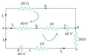
At junction a, current in equals current out: \(I_3 = I_1 + I_2\), written straight onto the figure. The two loop equations are there too — \(-30I_1 – 41I_3 + 45 = 0\) and \(-30I_1 + 21I_2 – 80 = 0\). Trace each loop with a finger while you read the signs, and copy this convention into your own solutions.
Figure 3.19, the Wheatstone bridge with values, is discussed in the bridge section above — return there to reread the arm labels and the galvanometer branch.
Key definitions and units at a glance
Built from the chapter’s own summary table (NCERT, p. 104) and the section text, each in one plain line.
| Quantity | Symbol | What it means | SI unit | Page |
|---|---|---|---|---|
| Electric current | \(I\) | Net charge crossing an area per unit time; a scalar | A | p. 82 |
| Charge | \(Q, q\) | Quantity of electricity | C | p. 104 |
| Voltage, potential difference | \(V\) | Work done per unit charge between two points | V | p. 104 |
| Electromotive force | \(\varepsilon\) | Work per unit charge done by a source; the open-circuit terminal voltage — a potential difference, not a force | V | p. 94 |
| Resistance | \(R\) | Ratio \(V/I\) for a conductor | \(\Omega\) | p. 83 |
| Resistivity | \(\rho\) | Material property in \(R = \rho l / A\) | \(\Omega\, \text{m}\) | p. 84 |
| Conductivity | \(\sigma\) | Reciprocal of resistivity, \(\sigma = 1/\rho\) | S | p. 85 |
| Current density | \(j\) | Current per unit area normal to the flow | A/m² | p. 84 |
| Drift speed | \(v_d\) | Steady average carrier speed due to the field, \(eE\tau/m\) | m/s | p. 86 |
| Relaxation time | \(\tau\) | Average time between successive collisions of an electron | s | p. 86 |
| Mobility | \(\mu\) | Drift speed per unit field, \(|v_d|/E\) | m²/Vs | p. 88 |
Mistakes students make in this chapter
The chapter’s own points to ponder (pp. 104–105) exist to correct exactly these. Learn them before you make them.
| Mistake | Correct rule | How to check your answer |
|---|---|---|
| “Current is a vector because it has a direction” | Current is a scalar: \(I = \mathbf{j} \cdot \Delta \mathbf{S}\) is a dot product, and currents never obey vector addition (NCERT, p. 104) | Add the currents at any junction as plain numbers — no parallelogram law |
| “\(V = IR\) is Ohm’s law” | \(V = IR\) defines resistance for any device; Ohm’s law is the claim that \(R\) is independent of \(V\), so the \(I\)–\(V\) plot is a straight line (NCERT, p. 104) | Plot \(I\) versus \(V\): a straight line through the origin means the device obeys Ohm’s law |
| “emf is a force” | emf is a potential difference, equal to the open-circuit terminal voltage of a cell (NCERT, p. 94) | Check the unit: volts, not newtons |
| “The bulb lights only when electrons from the switch reach it” | The field establishes a local electron drift almost instantly, so current starts everywhere at once (Example 3.2(a), NCERT, p. 88) | Notice the lamp comes on as soon as the switch closes, although drift speeds are about a millimetre per second |
| “Electrons must keep accelerating in the field” | Collisions reset the velocity; on average the electrons keep a steady drift speed (Example 3.2(b), NCERT, p. 88) | Compare \(v_d\) with thermal speeds — drift is far smaller and constant, not growing |
| “All free electrons drift together in one direction” | The drift is a tiny systematic motion superposed on large random thermal motion (Example 3.2(d), NCERT, p. 88) | Drift speed is about \(10^{-5}\) of thermal speeds at ordinary temperatures, yet the current is large because the electron density is enormous |
| “A negative current from Kirchhoff’s rules means an error” | A negative value means the true current flows opposite to the drawn arrow (NCERT, p. 97) | Keep the magnitude, reverse the arrow, and re-check that the loop equation still balances |
Problem types the chapter builds
The examples and exercises drill a small set of numerical skills. Revise by skill, and you cover the whole chapter.
| Problem type | Formula it leans on | Where the book practises it |
|---|---|---|
| Drift speed from current, density and area | \(I = neAv_d\) | Example 3.1 (p. 87); Exercise 3.9 (p. 106) |
| Terminal voltage and load current of a cell | \(I = \varepsilon/(R + r)\), \(V = \varepsilon – Ir\) | Exercises 3.1 and 3.2 (p. 105); Exercise 3.8 (p. 106) |
| Temperature coefficient of resistance | \(\rho_T = \rho_0[1 + \alpha(T – T_0)]\) | Examples 3.3, 3.4 (pp. 91–92); Exercises 3.3, 3.5, 3.6 (pp. 105–106) |
| Resistivity from wire dimensions | \(R = \rho l / A\) | Exercise 3.4 (p. 106) |
| Branch currents by Kirchhoff’s rules | Junction rule and loop rule | Example 3.6 (p. 99); Exercise 3.7 (p. 106, Fig. 3.20) |
| Wheatstone bridge balance | \(R_2/R_1 = R_4/R_3\) | Example 3.7 (p. 101); SUMMARY (p. 104) |
Fig. 3.20 is the network for Exercise 3.7 — the no-symmetry case to practise after Example 3.6. Assign each branch a current, apply the junction rule first to cut the number of unknowns, then write as many independent loops as you have unknowns.
One honest note: textbook contents and the examinable syllabus are not always identical — check the current official CBSE syllabus on cbse.gov.in before you decide what to revise in depth.
Chapter recap: the arguments in order
The book closes with its own summary (NCERT, pp. 102–104). Here it is in our words, as a chain you can say back the night before.
- Current is the net charge passing per unit time through a given area.
- A steady current needs a closed circuit and a source; the source’s work per unit charge is the emf — a potential difference in open circuit, not a force.
- Ohm’s law: \(V \propto I\), or \(V = RI\), with \(1\ \Omega = 1\ \text{V/A}\).
- Resistance of a conductor is \(R = \rho l/A\), with resistivity \(\rho\) a material property.
- Resistivity spans a huge range: metals \(10^{-8}\) to \(10^{-6}\ \Omega\, \text{m}\); insulators like glass and rubber \(10^{22}\) to \(10^{24}\) times larger; semiconductors in between.
- Carriers are electrons in most solids and ions in ionic crystals and electrolytes; current density is \(\mathbf{j} = nq\mathbf{v}_d\).
- Collisions give a steady drift: \(v_d = eE\tau/m\), so \(\rho = m/(ne^2\tau)\).
- The temperature coefficient \(\alpha\) measures the fractional rise in resistivity per degree over the linear range; and Ohm’s law fails in three distinct ways — nonlinearity, sign dependence, and non-uniqueness.
- With internal resistance, the external voltage is \(V_{ext} = \varepsilon R/(R + r)\).
- Kirchhoff’s junction rule conserves charge, the loop rule makes potential changes sum to zero around a loop, and the Wheatstone null condition is \(R_1/R_2 = R_3/R_4\).
Related resources
This listing is maintained for the 2026-27 academic session using the NCERT textbook information available to us. NCERT remains the authority for confirming the latest edition.
From here you can move forward or back through Class 12 Physics:
- the NCERT Class 12 Physics book page lists every chapter of Part I and Part II;
- the Class 12 hub gathers notes for all your Class 12 subjects;
- Chapter 2: Electrostatic Potential and Capacitance is the chapter just before this one, where the story of charges at rest ends;
- Chapter 4: Moving Charges and Magnetism comes next — this chapter itself points forward to it when it notes that the ampere is defined through the magnetic effects of currents (NCERT, p. 82);
- the CBSE notes home is the main index of every chapter page on the site.
The official NCERT website holds the current editions of every textbook, including the physics text this chapter comes from.
Sources and data verification
- The counts, figures and page references on this page describe the NCERT Class 12 Physics Part I textbook, Chapter 3 Current Electricity, printed pages 80–106 of the current edition.
- This page covers the textbook chapter and its contents — not the CBSE examination scheme, sample papers or marking patterns.
- It is maintained for the current academic session using the NCERT information available to us.
- NCERT settles textbooks, editions and official PDFs; CBSE settles the curriculum, syllabus and examinations.
Reference: NCERT Class 12 Physics textbook, chapter 3, official edition on ncert.nic.in.
Frequently asked questions
Why is current called a scalar when it flows in a definite direction?
Because current is defined as the scalar product of two vectors. The current through an area is \(I = \mathbf{j} \cdot \Delta \mathbf{S}\), a dot product of the current density and the area vector, and a dot product is a number, not a vector.
Currents also fail vector addition: at a junction they add as ordinary numbers, however the wires bend (NCERT, p. 104).
If drift speed is only about a millimetre per second, why does the bulb light almost as soon as the switch is closed?
Because the current starts when the field reaches the electrons, not when an electron arrives from the far end.
The electric field establishes a local electron drift throughout the circuit almost instantly (at a speed comparable to the speed of light), so a current begins everywhere at once; it only takes a little while to reach its steady value (Example 3.2(a), NCERT, p. 88).
Is V = IR the same thing as Ohm’s law?
No. The equation \(V = IR\) defines resistance, and it can be applied to any conducting device, whether or not the device obeys Ohm’s law. Ohm’s law is the stronger claim that \(R\) is independent of \(V\), so the \(I\)–\(V\) plot is a straight line. A diode’s graph bends, yet you can still call \(V/I\) its resistance (NCERT, p. 104).
Why is electrical power transmitted over long distances at very high voltage?
Because cable loss falls as the square of the voltage. For a fixed delivered power \(P\), the cables dissipate \(P_c = P^2R_c/V^2\); raise the voltage and the current \(I = P/V\) falls, and the loss, which scales with \(I^2\), falls steeply.
Lines therefore run at enormous voltages, and a transformer steps the voltage down near homes and factories (NCERT, p. 93).
What does a negative value of current mean in a Kirchhoff’s rules solution?
It means the real current flows opposite to the arrow you drew — not that you made an arithmetic error. Kirchhoff’s rules accept any consistent labelling; if a current comes out negative, read that branch as having magnitude \(|I|\) in the reverse direction and continue with the solution (NCERT, p. 97).
Why is the emf of a cell called an electromotive force if it is not a force?
The name is historical, kept because the phenomenon was not understood when it was coined. The emf \(\varepsilon\) is actually a potential difference — the work done per unit charge by the source in moving charge from one terminal to the other — and its unit is the volt, the same as any potential difference.
It is not a force measured in newtons (NCERT, p. 94).
Explore Class 12 Physics Books
Class 12 Physics on LearnCBSE:
Related chapters: