
This page holds the official electromagnetic induction class 12 chapter — NCERT Class 12 Physics Part I, Chapter 6 — and a clear walkthrough of what it teaches. The chapter answers one question: how a changing magnetic field generates an electric current. That single idea runs generators, transformers and the power grid.
The official NCERT PDF (2026-27 reprint of Physics Part I, printed pages 153–176) is right below. Everything after it explains the chapter section by section, with the page numbers and figures from your own book.
Download Electromagnetic Induction Class 12 PDF
The official file is hosted by NCERT itself, and the link below opens it directly. Download the NCERT Class 12 Physics Chapter 6 Electromagnetic Induction PDF to read the chapter in its printed layout — all figures, worked examples and the complete exercise set — exactly as it appears in the current NCERT reprint of Physics Part I.
If you want to confirm the edition or open other chapters, browse the NCERT textbook portal.
| What the chapter holds | Count | Where it is used |
|---|---|---|
| Printed pages | 23 | |
| Sections in the chapter | 10 | |
| Figures with NCERT captions | 11 | |
| Tables | 1 | |
| Worked examples | 3 | solved step by step in our NCERT Solutions |
| Exercise questions | 8 | answered in our NCERT Solutions |
| Official NCERT PDF | Download the chapter PDF | the chapter exactly as NCERT publishes it |
Chapter 6 at a Glance: What Is Inside the PDF
The chapter contents table below summarises the size and shape of the file — how many sections, diagrams, worked examples and exercise questions it holds. Keep it open while you read; the list under it names each section in the order the book presents it.
The chapter is organised in this order:
- 6.1 Introduction
- 6.2 The Experiments of Faraday and Henry
- 6.3 Magnetic Flux
- 6.4 Faraday’s Law of Induction
- 6.5 Lenz’s Law and Conservation of Energy
- 6.6 Motional Electromotive Force
- 6.7 Inductance
- 6.8 AC Generator
- Summary
- Points to Ponder
- Exercises
What This Chapter Covers and Why It Matters
In the early nineteenth century, Oersted and Ampère showed that an electric current produces a magnetic field — a compass needle deflects near a current-carrying wire. Around 1830, Faraday in England and Henry in the USA asked the reverse question: can a magnetic field produce a current?
The answer is yes, but only while the field is changing, and this chapter is the full working out of that answer (NCERT, p. 155).
The book records Faraday’s famous reply when asked what his discovery was good for: “What is the use of a new born baby?” His point was that the practical uses would come later — generators and transformers are those uses (NCERT, p. 155).
One line of preview, and everything else in the chapter is detail:
- The three experiments (p. 155–156): three set-ups that all induce current, each a different way of changing magnetic flux.
- Magnetic flux (p. 157): the quantity \( \Phi_B = BA\cos\theta \) whose change drives everything.
- Faraday’s law (p. 158): the induced emf equals the negative rate of change of flux.
- Lenz’s law (p. 160): the induced current opposes the change that created it — conservation of energy in disguise.
- Motional emf (p. 162): a rod moving through a field develops \( \varepsilon = Blv \) across its ends.
- Inductance (p. 165–168): coils oppose changes in their own current (self-inductance) and in a neighbour’s (mutual inductance).
- AC generator (p. 170): rotating a coil in a field turns Faraday’s law into alternating current.
Key Concepts in Electromagnetic Induction Class 12
The Three Experiments of Faraday and Henry
All three experiments in §6.2 are the same idea wearing three costumes: change the magnetic flux through a coil and a current appears in it. Keep that sentence in mind and the experiments stop being three separate facts.
- Experiment 6.1 (p. 155): a coil is connected to a galvanometer. Push the north pole of a bar magnet towards it and the pointer deflects — but only while the magnet moves. Pull the magnet away and the deflection reverses. Move the magnet faster and the deflection grows. Moving the coil instead of the magnet gives the same result, so it is relative motion that matters.
- Experiment 6.2 (p. 156): the bar magnet is replaced by a second coil carrying a steady current. That coil behaves like a magnet: moving it toward or away from the test coil induces a current, with the deflection reversing on the way out.
- Experiment 6.3 (p. 156): both coils are held stationary. Press the tapping key and the galvanometer kicks momentarily; hold the key and nothing happens; release it and there is an opposite kick. An iron rod inserted along the axis strengthens the deflection dramatically. Relative motion is not an absolute requirement — a changing current is enough.
The three experiments teach one lesson (NCERT, p. 157): an emf appears whenever the magnetic flux through the circuit changes, and for no other reason.
Magnetic Flux and the Area Vector
Magnetic flux is the quantity you must change before anything in this chapter happens — it is, roughly, the amount of magnetic field threading a surface.
For a plane of area \( A \) in a uniform field \( B \), \[ \Phi_B = \mathbf{B}\cdot\mathbf{A} = BA\cos\theta \tag{6.1} \]
where \( \theta \) is the angle between the field vector \( \mathbf{B} \) and the area vector \( \mathbf{A} \) — the normal drawn perpendicular to the plane. This is where students stumble: \( \theta \) is not the angle between the field and the plane itself.
Flux is maximum when the plane faces the field (\( \theta = 0^\circ \)) and zero when the plane is edge-on (\( \theta = 90^\circ \)).
Flux is a scalar quantity, measured in weber (Wb) or tesla metre squared (T m\(^2\)) (NCERT, p. 157). When the field varies from point to point, Eq. (6.2) extends the idea by summing \( \mathbf{B}_i \cdot \mathrm{d}\mathbf{A}_i \) over every small area element of the surface.
Faraday’s Law of Induction
The law is one sentence: the induced emf equals the time rate of change of magnetic flux. Notice what is absent — nothing about how large the field is, only how fast it changes.
Mathematically, the induced emf is \[ \varepsilon = -\frac{\mathrm{d}\Phi_B}{\mathrm{d}t} \tag{6.3} \]
and for a closely wound coil of \( N \) turns, where the same flux links every turn, \[ \varepsilon = -N\frac{\mathrm{d}\Phi_B}{\mathrm{d}t} \tag{6.4} \]
The minus sign encodes the direction of the emf — that is Lenz’s law, the next section. If the circuit is closed, a current \( I = \varepsilon/R \) flows, where \( R \) is the circuit resistance (NCERT, p. 158). Flux can be changed by varying B, A or \( \theta \): shrinking a loop, stretching it, or rotating it in a field all work.
A steady flux, however large, induces nothing — NCERT’s Example 6.2 makes the point by noting that the Earth’s steady field adds no emf (p. 159).
Lenz’s Law and Conservation of Energy
Lenz’s law answers the direction question: the polarity of the induced emf is such that it tends to produce a current which opposes the change in flux — not the flux itself (NCERT, p. 160).
Watch it work with an approaching north pole. Flux into the coil is increasing, so the induced current must oppose that increase. It flows counter-clockwise as seen from the magnet, making its own north pole face the approaching north pole — a repulsion, as if the coil were pushing the magnet back.
When the north pole is withdrawn, flux decreases, so the induced current reverses, its south pole now facing the receding magnet and attracting it (NCERT, p. 160).
Why must it be this way? Suppose the current aided the change instead. A gentle push on the magnet would then be reinforced by the coil, accelerating forever with no energy input — a perpetual-motion machine, which violates conservation of energy.
With Lenz’s law, you do mechanical work pushing the magnet against the repulsion, and that work reappears as Joule heating in the coil (NCERT, p. 161). In an open circuit the emf still exists across the open ends; only the current is missing because the path is broken.
Motional EMF and the Lorentz Force
Move a conductor through a magnetic field and its free charges feel a magnetic force — that is motional emf, the easiest way to make Faraday’s law happen in a machine.
Consider a rod of length \( l \) sliding on rails at speed \( v \), with the field \( B \) normal to the plane of the loop. The flux enclosed is \( \Phi_B = Blx \), where \( x \) is the remaining length of the loop. Differentiating, \[ \varepsilon = -\frac{\mathrm{d}\Phi_B}{\mathrm{d}t} = Blv \tag{6.5} \]
since \( \mathrm{d}x/\mathrm{d}t = -v \). The book gives a second route to the same answer: each charge \( q \) in the moving rod experiences a Lorentz force \( qvB \) directed along the rod, and the work done per unit charge is \( W/q = qvBl/q = Blv \) (NCERT, p. 162–163).
The subtle case is a stationary conductor in a changing field. With \( v = 0 \), the magnetic part of the Lorentz force is zero, so the emf must come from an induced electric field:
\[ \mathbf{F} = q(\mathbf{E} + \mathbf{v}\times\mathbf{B}) = q\mathbf{E} \tag{6.6} \]
This is the deep result: a time-varying magnetic field generates an electric field (NCERT, p. 163). For a rod rotating about one end, the speed varies along its length, so you integrate \( \mathrm{d}\varepsilon = Bv\,\mathrm{d}r \) with \( v = \omega r \) to get \( \varepsilon = \frac{1}{2}B\omega R^2 \) — NCERT’s Example 6.6 works it to 157 V (p. 164).
Mutual Inductance
Put two coils near each other: a changing current in one induces an emf in the other. The constant that ties them together is mutual inductance \( M \).
By definition, the flux linkage in coil 1 is proportional to the current in coil 2:
\[ N_1\Phi_1 = M_{12}I_2 \tag{6.7} \]
For two long coaxial solenoids of the same length \( l \), with the inner one of radius \( r_1 \) having \( n_1 \) turns per unit length and the outer one \( n_2 \), the geometry gives \[ M_{12} = \mu_0 n_1 n_2 \pi r_1^2 l \tag{6.9} \]
and doing the calculation the other way round gives the same value, so \( M_{12} = M_{21} \) — a general result far beyond these solenoids (NCERT, p. 166). If a medium of relative permeability \( \mu_r \) fills the space, multiply by \( \mu_r \). Mutual inductance depends on the separation and relative orientation of the coils (p. 167).
When the current in coil 2 varies, the emf induced in coil 1 is \[ \varepsilon_1 = -M\frac{\mathrm{d}I_2}{\mathrm{d}t} \]
The unit of inductance, in honour of Joseph Henry, is the henry (H).
Self-Inductance and Magnetic Energy
A coil is its own neighbour: a changing current induces an emf in the same coil that carries it. Self-inductance \( L \) is the measure of that opposition.
The flux linkage of the coil is proportional to its own current, \[ N\Phi_B = LI \tag{6.13} \]
so a changing current induces a self-emf, \[ \varepsilon = -L\frac{\mathrm{d}I}{\mathrm{d}t} \tag{6.14} \]
This back emf opposes any change — increase or decrease — of the current. The book calls \( L \) the electromagnetic analogue of mass: it plays the role of inertia, resisting changes in current just as mass resists changes in velocity (NCERT, p. 168).
For a long solenoid of cross-sectional area \( A \), length \( l \) and \( n \) turns per unit length, \[ L = \mu_r\mu_0 n^2 A l \tag{6.16} \]
The work done building up the current is stored as magnetic energy, \[ W = \frac{1}{2}LI^2 \tag{6.17} \]
and the energy per unit volume of a magnetic field is \( u_B = B^2/2\mu_0 \) — the magnetic twin of the capacitor’s \( u_E = \frac{1}{2}\varepsilon_0 E^2 \) (NCERT, p. 169–170).
The AC Generator
The AC generator is Faraday’s law built as a machine: rotate a coil in a field and the flux keeps changing, so a sinusoidal emf comes out of the ends.
As the coil rotates with constant angular speed \( \omega \), the angle between \( \mathbf{B} \) and the area vector grows as \( \theta = \omega t \). The flux is then \[ \Phi_B = BA\cos\omega t \]
and Faraday’s law differentiates it:
\[ \varepsilon = -N\frac{\mathrm{d}\Phi_B}{\mathrm{d}t} = NBA\omega\sin\omega t \tag{6.19} \]
The peak value is \( \varepsilon_0 = NBA\omega = NBA(2\pi\nu) \), where \( \nu \) is the frequency of revolution (NCERT, p. 171). The sine changes sign every half cycle, so the current reverses direction periodically — that is why it is called alternating current.
Slip rings and brushes carry the rotating coil’s output to the external circuit, and in India the standard frequency is 50 Hz (p. 172).
Formula Map: Which Equation to Use When
The whole chapter runs on a small set of relations. In the table, \( B \) is the magnetic field, \( A \) the area, \( N \) the number of turns, \( l \) a conductor length, \( v \) a speed, \( n \) turns per unit length, \( \mu_0 \) the permeability of free space, \( \mu_r \) the relative permeability, \( \omega \) the angular speed and \( \nu \) the frequency.
| Quantity | Formula | Symbols | SI unit | Where it appears |
|---|---|---|---|---|
| Magnetic flux | \( \Phi_B = BA\cos\theta \) | \( \theta \) = angle between \( \mathbf{B} \) and area vector | weber (Wb) | p. 157 |
| Faraday’s law, \( N \) turns | \( \varepsilon = -N\,\mathrm{d}\Phi_B/\mathrm{d}t \) | \( \varepsilon \) = induced emf, \( t \) = time | volt (V) | p. 158 |
| Motional emf | \( \varepsilon = Blv \) | \( l \) = rod length, \( v \) = speed, all mutually perpendicular | volt (V) | p. 162 |
| Mutual inductance | \( N_1\Phi_1 = M_{12}I_2 \), \( \varepsilon_1 = -M\,\mathrm{d}I_2/\mathrm{d}t \) | \( M \) = mutual inductance | henry (H) | p. 166–167 |
| Self-inductance | \( N\Phi_B = LI \), \( \varepsilon = -L\,\mathrm{d}I/\mathrm{d}t \) | \( L \) = self-inductance | henry (H) | p. 168 |
| Solenoid self-inductance | \( L = \mu_r\mu_0 n^2 A l \) | \( n \) = turns per unit length | henry (H) | p. 168 |
| Magnetic energy | \( W = \frac{1}{2}LI^2 \); density \( u_B = B^2/2\mu_0 \) | \( I \) = current | joule (J) | p. 169–170 |
| AC generator peak emf | \( \varepsilon_0 = NBA\omega = NBA(2\pi\nu) \) | \( \omega \) = angular speed | volt (V) | p. 171 |
Put the two inductances side by side and the difference is easy to hold onto:
| Property | Mutual inductance \( M \) | Self-inductance \( L \) |
|---|---|---|
| Defining equation | \( N_1\Phi_1 = MI_2 \) | \( N\Phi_B = LI \) |
| What it links | flux in one coil to current in a nearby coil | flux in a coil to its own current |
| Induced emf | \( \varepsilon_1 = -M\,\mathrm{d}I_2/\mathrm{d}t \) | \( \varepsilon = -L\,\mathrm{d}I/\mathrm{d}t \) (back emf) |
| SI unit | henry (H) | henry (H) |
| Physical meaning | couples two circuits; \( M_{12} = M_{21} \) always | electromagnetic inertia, the analogue of mass |
| Depends on | geometry, separation and orientation of the coils (p. 167) | geometry and permeability of the medium (p. 168) |
Figure Walkthrough: Reading the NCERT Diagrams
The diagrams carry this chapter better than the equations do — each one is a different way of changing flux. Work through them in order and the whole chapter becomes a single idea. The NCERT page is cited beside each group.
The Experiment Diagrams: Figures 6.1, 6.2 and 6.3
These three set-ups are the evidence the whole chapter rests on. Read them as three ways of changing the flux through the same test coil.
This is the replacement that turns Experiment 6.1 into Experiment 6.2. A steady current in coil C₂ produces a steady magnetic field, so C₂ behaves exactly like the bar magnet; moving C₂ towards C₁ changes the flux through C₁ the same way the magnet did (NCERT, p. 155).
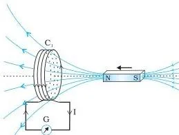
The galvanometer G is the detector: it deflects only while the magnet is in motion, reverses when the magnet is pulled away, and kicks harder when the magnet moves faster. Holding the magnet still leaves the flux constant, so the pointer sits at zero (NCERT, p. 155).
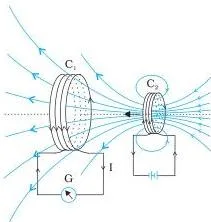
The steady current in C₂ makes a steady field, so the only way to change the flux through C₁ is to move one coil relative to the other. Away or towards, the pointer deflects while the motion lasts — relative motion between the coils is what induces the current (NCERT, p. 156).
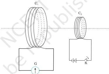
Nothing moves in this set-up — yet current still appears. Pressing the key grows the current in C₂ from zero to its full value, changing the flux through C₁ and producing a momentary kick; holding the key keeps the flux steady, so nothing flows; releasing the key collapses the flux and gives an opposite kick.
The iron rod multiplies the deflection because it concentrates the field lines (NCERT, p. 156).
Flux Diagrams: Figures 6.4 and 6.5
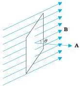
This diagram fixes where the angle lives. The area vector \( \mathbf{A} \) is the arrow drawn normal to the plane, and \( \theta \) sits between that normal and the field \( \mathbf{B} \). Face the plane into the field and \( \theta = 0^\circ \), giving maximum flux; turn it edge-on and \( \theta = 90^\circ \), giving zero (NCERT, p. 157).
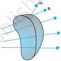
When the field differs from point to point you cannot multiply one value of \( B \) by the whole area. The figure shows the surface broken into small elements, each carrying its own \( \mathbf{B}_i \) and \( \mathrm{d}\mathbf{A}_i \); the flux is the sum \( \sum \mathbf{B}_i\cdot\mathrm{d}\mathbf{A}_i \) (Eq. 6.2, NCERT, p. 157).
Lenz’s Law on Moving Loops: Figure 6.7
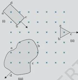
Practise the direction rule on all three shapes (NCERT, p. 161). A loop entering the field has increasing flux, so the induced current must oppose entry — the rectangular loop carries current along the path bcdab.
A loop leaving the field has decreasing flux, so the current tries to hold the flux in — the triangular loop uses bacb and the irregular loop cdabc. And note the quiet case: while a loop is wholly inside or wholly outside the field, its flux is constant and there is no induced current at all.
Motional EMF: Figure 6.10
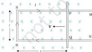
Trace the circuit: the rod PQ slides left, so the length \( x = RQ \) shrinks and the enclosed area \( lx \) falls. With \( \Phi_B = Blx \) and \( \mathrm{d}x/\mathrm{d}t = -v \), Faraday’s law gives \( \varepsilon = Blv \).
The length involved is \( l = RS \), the speed \( v \) is the rate at which \( x \) changes, and the current direction shown follows Lenz’s law — the shrinking flux must be opposed (NCERT, p. 162).
Mutual Inductance: Figure 6.12
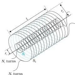
This geometry is where the formula for \( M \) comes from (NCERT, p. 166). The inner solenoid has radius \( r_1 \) and \( n_1 \) turns per unit length; the outer has \( n_2 \).
A current \( I_2 \) in the outer solenoid sets up a field \( \mu_0 n_2 I_2 \) threading the inner one, and counting the flux linkage turn by turn gives \( M_{12} = \mu_0 n_1 n_2 \pi r_1^2 l \).
Reversing the roles gives the same expression, which is why \( M_{12} = M_{21} \) — the equality that lets you compute the easy direction and trust it for the hard one.
AC Generator: Figures 6.13 and 6.14
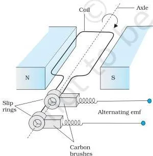
The machine diagram names the parts (§6.8, NCERT, p. 170). The armature coil is mounted on a rotor shaft and rotated in a uniform field with its axis of rotation perpendicular to the field. The coil ends are connected to the external circuit through slip rings and brushes, so the rotating coil can keep delivering its changing output.
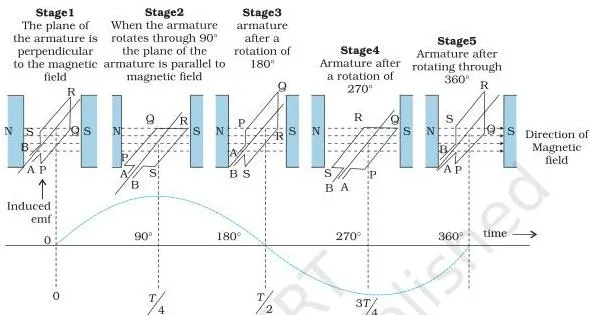
This graph is Eq. (6.19) drawn. The emf peaks at \( \theta = 90^\circ \) and \( 270^\circ \), where the flux is changing fastest, and passes through zero at \( 0^\circ \) and \( 180^\circ \), where the flux momentarily stops changing. Because the sine wave changes sign, the polarity reverses twice per rotation — alternating current (NCERT, p. 171–172).
Definitions You Need for Electromagnetic Induction Class 12
Before the formulas, make sure the words are fixed — answers are marked on them. Each term below is in plain language, with its unit where one exists.
| Term | Plain meaning | Unit |
|---|---|---|
| Electromagnetic induction (p. 153) | generating an electric current by varying the magnetic field linked with a circuit | — |
| Magnetic flux (p. 157) | \( \Phi_B = BA\cos\theta \), the measure of field threading a surface; a scalar | weber (Wb) |
| Flux linkage (p. 165) | \( N\Phi_B \) for a closely wound coil — the same flux links every turn, so the total is \( N \) times the single-turn flux | Wb (per coil) |
| Induced emf (p. 158) | the voltage produced by a changing flux; \( \varepsilon = -N\,\mathrm{d}\Phi_B/\mathrm{d}t \) | volt (V) |
| Motional emf (p. 162) | emf produced by moving a conductor through a field; \( \varepsilon = Blv \) | volt (V) |
| Mutual inductance (p. 166) | ratio of flux linkage in one coil to the current in a neighbouring coil; \( N_1\Phi_1 = M_{12}I_2 \) | henry (H) |
| Self-inductance and back emf (p. 168) | \( L \) from \( N\Phi_B = LI \); the self-induced emf \( -L\,\mathrm{d}I/\mathrm{d}t \) opposes any change of current | henry (H) |
Common Mistakes in Electromagnetic Induction and How to Avoid Them
These are the errors the chapter’s own worked examples and Points to Ponder are guarding against. Name them now and you will not make them at midnight.
| Mistake | Correct rule | How to check your answer |
|---|---|---|
| Expecting a current from a stationary magnet, however strong | Only a changing flux induces emf: \( \varepsilon = -N\,\mathrm{d}\Phi_B/\mathrm{d}t \). A steady field, however large, gives \( \varepsilon = 0 \) (NCERT, p. 161, Ex. 6.5a) | Ask: is anything changing — \( B \), \( A \) or \( \theta \)? If none, the emf is zero. |
| Using the angle between the field and the plane of the coil | \( \theta \) is between \( \mathbf{B} \) and the area vector \( \mathbf{A} \), the normal to the plane (NCERT, p. 157) | Draw the coil’s normal; the angle from that line to \( \mathbf{B} \) is \( \theta \). |
| Forgetting to multiply by \( N \) for a coil | Each turn links the flux, so the total emf is \( -N\,\mathrm{d}\Phi_B/\mathrm{d}t \) (NCERT, p. 158) | Check the given turns count; a 200-turn coil gives 200 times the single-turn emf. |
| Thinking an open circuit has no induced emf | The emf still develops across the open ends; only the current is zero because the path is broken (NCERT, p. 160) | An open loop still shows voltage across its ends; current needs a closed path. |
| Expecting changing electric flux to induce current | Faraday’s law is about magnetic flux only; electric flux induces nothing (NCERT, p. 161, Ex. 6.5b) | Identify what is changing; for induced current it must be magnetic flux. |
| Expecting current while a loop is wholly inside or outside the field | With the whole loop in (or out), its flux is constant, so there is no emf (NCERT, p. 161, Ex. 6.4) | Find the part crossing the field boundary; that part generates the emf. |
How to Prepare This Chapter for Your Exams
Numericals in this chapter are almost all one pattern: something changes, so flux changes, so an emf appears. Run the same five-step recipe every time.
- Write the flux formula \( \Phi_B = BA\cos\theta \) with the correct area and the correct angle.
- Find the initial flux.
- Find the final flux.
- Take the magnitude of the change, divide by the time \( \Delta t \), and multiply by the number of turns \( N \).
- Divide by the resistance to get the current: \( I = \varepsilon/R \).
Here is the recipe worked on a problem with fresh numbers — a 200-turn coil of radius 5 cm and resistance 4 Ω, placed with its plane perpendicular to a uniform 0.2 T field, then rotated through 180° in 0.1 s.
Step 1: Write the flux formula.
The area is \( A = \pi r^2 \), and the angle must be measured to the area vector.
\[ A = \pi(0.05)^2 = 7.85\times10^{-3}\ \text{m}^2 \]
Step 2: Find the initial flux.
The plane starts perpendicular to the field, so \( \theta = 0^\circ \).
\[ \Phi_i = BA\cos 0^\circ = 0.2 \times 7.85\times10^{-3} = 1.57\times10^{-3}\ \text{Wb} \]
Step 3: Find the final flux after rotation through \( 180^\circ \).
Now \( \theta = 180^\circ \).
\[ \Phi_f = BA\cos 180^\circ = -1.57\times10^{-3}\ \text{Wb} \]
Step 4: Take the change in flux and divide by the time.
\[ |\Delta\Phi| = 3.14\times10^{-3}\ \text{Wb},\qquad \frac{|\Delta\Phi|}{\Delta t} = \frac{3.14\times10^{-3}}{0.1} = 3.14\times10^{-2}\ \text{Wb/s} \]
Step 5: Multiply by the number of turns \( N = 200 \).
\[ |\varepsilon| = N\frac{|\Delta\Phi|}{\Delta t} = 200 \times 3.14\times10^{-2} = 6.28\ \text{V} \]
Step 6: Divide by the resistance to get the current.
\[ I = \frac{\varepsilon}{R} = \frac{6.28}{4} = 1.57\ \text{A} \]
Final answer: average emf \( \approx 6.28\ \text{V} \) and average current \( \approx 1.57\ \text{A} \). The word average matters — instantaneous values depend on how the rotation speed varies during the 0.1 s, exactly as NCERT’s own Example 6.3 notes for its numbers (NCERT, p. 159).
The end-of-chapter exercises map cleanly onto the same formulas. Know which weapon to reach for:
| Exercise | What it tests | Formula to reach for |
|---|---|---|
| 6.3 | flux through a small loop inside a solenoid while the solenoid current changes steadily | \( B = \mu_0 nI \), then \( \varepsilon = \mathrm{d}\Phi/\mathrm{d}t \) |
| 6.4 | rectangular loop leaving a uniform field with a small cut | motional emf \( \varepsilon = Blv \) by area change |
| 6.5 | metallic rod rotating about one end | \( \varepsilon = \frac{1}{2}B\omega R^2 \) |
| 6.6 | straight wire falling through the Earth’s horizontal field | \( \varepsilon = Blv \) with \( l = 10\ \text{m} \), \( v = 5.0\ \text{m/s} \) |
| 6.7 | current falls from 5.0 A to zero in 0.1 s, average emf 200 V | self-inductance: \( |\varepsilon| = L\,|\Delta I|/\Delta t \) |
| 6.8 | adjacent coils of mutual inductance 1.5 H | flux-linkage change: \( \Delta(N\Phi) = M\,\Delta I \) |
Two of those check out in one line each: exercise 6.7 gives \( L = 200 \times 0.1/5 = 4\ \text{H} \), and exercise 6.8 gives a flux-linkage change of \( 1.5 \times 20 = 30\ \text{Wb} \). One honest warning before you revise: textbook contents and the examinable syllabus are not always identical — check the current official syllabus before assuming any section is tested.
Electromagnetic Induction Class 12 Quick Revision
This is the chapter’s own summary restated in plain words (NCERT, p. 173–174). Read it the night before, then check each bullet against the flagging sections above.
- Flux: \( \Phi_B = BA\cos\theta \), where \( \theta \) is between \( \mathbf{B} \) and the area vector; it is a scalar measured in webers.
- Faraday’s law: \( \varepsilon = -N\,\mathrm{d}\Phi_B/\mathrm{d}t \); a closed circuit carries \( I = \varepsilon/R \).
- Lenz’s law: the induced current opposes the change in flux; the minus sign is this law, and it is conservation of energy in disguise.
- Motional emf: a rod of length \( l \) moving at speed \( v \) normal to \( B \) develops \( \varepsilon = Blv \).
- Inductance: the ratio of flux linkage to current; flux linkage \( N\Phi \) is proportional to \( I \).
- Mutual inductance: \( \varepsilon_1 = -M\,\mathrm{d}I_2/\mathrm{d}t \), with \( M_{12} = M_{21} \) always.
- Self-inductance: \( \varepsilon = -L\,\mathrm{d}I/\mathrm{d}t \); \( L \) is the electrical inertia of the coil.
- Solenoid: \( L = \mu_r\mu_0 n^2Al \).
- Magnetic energy: \( W = \frac{1}{2}LI^2 \), with energy density \( B^2/2\mu_0 \).
- AC generator: \( \varepsilon = NBA(2\pi\nu)\sin(2\pi\nu t) \), peak \( \varepsilon_0 = NBA\omega \).
Related NCERT Class 12 Physics Chapters
Magnetism and Matter (Chapter 5) sets up the magnetic field ideas this chapter then changes. The Class 12 Physics notes hub gathers the whole subject, the Class 12 notes hub covers every subject, and the main CBSE notes directory holds the entire site.
Alternating Current (Chapter 7) starts exactly where this chapter stops: it takes the sinusoidal emf of §6.8 and asks what resistors, inductors and capacitors do with it, so make Eq. (6.19) comfortable before moving on. In the broader Class 12 course, later chapters such as Nuclei are also waiting in the same notes hub.
Sources and Data Verification
All facts, page numbers and figure captions on this page come from the same source you can check: the NCERT textbook itself. Four points to be precise about what this page is.
- The contents, figures, page numbers and formulas describe the NCERT Class 12 Physics Part I textbook, Chapter 6 (Electromagnetic Induction), 2026-27 reprint, as published on ncert.nic.in.
- This page covers that single chapter only — not Physics Part II, not other subjects, and not the exercises of other chapters.
- The page is maintained for the current session from the NCERT information available to us.
- NCERT settles textbook editions and PDFs; CBSE settles the curriculum, syllabus and examinations.
Electromagnetic Induction Class 12: Frequently Asked Questions
Why is no current induced when a magnet is held stationary inside a coil?
Because Faraday’s law responds only to change: \( \varepsilon = -\mathrm{d}\Phi_B/\mathrm{d}t \). With the magnet held still, the flux through the coil is constant, so \( \mathrm{d}\Phi_B/\mathrm{d}t = 0 \) and no emf appears — Experiment 6.1 shows the deflection lasting only while the magnet moves (NCERT, p. 155).
A stronger magnet raises the flux but does not change it, so it still induces nothing (NCERT, p. 161).
What is the difference between magnetic flux and flux linkage?
Magnetic flux \( \Phi_B = BA\cos\theta \) is the flux through a single turn — a scalar in webers describing how much field threads the surface (NCERT, p. 157). Flux linkage is \( N\Phi_B \) for a closely wound coil of \( N \) turns: because the same flux links every turn, the total is \( N \) times the single-turn flux (NCERT, p. 165).
Faraday’s law for a coil is written with the linkage: \( \varepsilon = -\mathrm{d}(N\Phi_B)/\mathrm{d}t \).
When is the motional emf formula \( \varepsilon = Blv \) valid?
When a rod of length \( l \) is normal to a uniform magnetic field \( B \) and moves with velocity \( v \) perpendicular to the field — so \( B \), \( l \) and \( v \) are mutually perpendicular (NCERT, p. 173). If \( v \) has a component along the rod, only the component perpendicular to both \( l \) and \( B \) contributes.
For a rod rotating about one end, the speed varies along the rod, so you integrate \( \mathrm{d}\varepsilon = Bv\,\mathrm{d}r \) and get \( \varepsilon = \frac{1}{2}B\omega R^2 \).
Why does Lenz’s law follow from conservation of energy?
If the induced current aided the flux change instead of opposing it, the system would accelerate on its own: a gentle push towards the coil would grow into ever-faster motion with no energy input — a perpetual-motion machine, which violates conservation of energy (NCERT, p. 160).
With Lenz’s law, you must do work pushing the magnet against the repulsive force, and that work is dissipated as Joule heating in the coil. That is where the energy goes.
What is back emf in self-induction?
When the current through a coil changes, the coil induces an emf in itself, \( \varepsilon = -L\,\mathrm{d}I/\mathrm{d}t \), that opposes any change — increase or decrease — of the current.
This self-induced emf is called the back emf, and \( L \), the self-inductance, is its measure; the book describes \( L \) as the electromagnetic analogue of mass, the electrical inertia of the coil (NCERT, p. 168).
How does an AC generator produce alternating current and why is the emf sinusoidal?
The coil rotates so the angle between \( \mathbf{B} \) and the area vector grows as \( \theta = \omega t \). The flux then varies as \( \Phi = BA\cos\omega t \), and Faraday’s law differentiates the cosine into a sine: \( \varepsilon = NBA\omega\sin\omega t \) (NCERT, p. 171).
The sine changes sign every half cycle, so the current reverses direction periodically — that is the alternating current. The emf is largest at \( \theta = 90^\circ \) and \( 270^\circ \), where the flux changes fastest, and zero at \( 0^\circ \) and \( 180^\circ \) (NCERT, p. 172); slip rings and brushes carry the rotating coil’s output to the external circuit.
Reference: NCERT Class 12 Physics textbook, chapter 6, official edition on ncert.nic.in.
Explore Class 12 Physics Books
Class 12 Physics on LearnCBSE:
Related chapters: