
These magnetism and matter class 12 notes compress the whole chapter into a revision-ready form: the bar magnet as a magnetic dipole, its field lines, torque and potential energy in a uniform field, the axial and equatorial field formulas, Gauss’s law of magnetism, and the H–M–χ chain that classifies dia-, para- and ferromagnetic materials.
Every idea carries its NCERT page, so you can verify from the source. They are part of our Class 12 Physics notes.
Use them the way an examiner would want: read one section, then try the worked numericals yourself before reading the steps. All formulas include units, and the comparison tables at the end are the fastest way to revise the night before the exam.
Short on time? Read the Chapter at a Glance below, then the one-page revision summary at the bottom. Jump straight to any topic from the contents.
Magnetism and Matter Class 12 Notes: Chapter at a Glance
The chapter builds in a strict order — each idea leans on the one before it (NCERT, p. 136–152).
- Bar magnet as a dipole — poles always come in pairs; field lines form closed loops (p. 137).
- Solenoid analogy — a bar magnet behaves like a solenoid of circulating currents (Ampere’s hypothesis) (p. 138).
- Dipole in a uniform field — net force zero; torque \( \boldsymbol{\tau} = \mathbf{m} \times \mathbf{B} \), energy \( U_m = -\mathbf{m}\cdot\mathbf{B} \) (p. 139).
- Far fields — axial \( B_A = \frac{\mu_0}{4\pi}\frac{2m}{r^3} \), equatorial \( B_E = -\frac{\mu_0}{4\pi}\frac{m}{r^3} \), via the electrostatic analogy (p. 140–141).
- Gauss’s law of magnetism — net flux through any closed surface is zero; no magnetic monopoles (p. 142).
- Magnetisation and intensity — \( M = m_{\text{net}}/V \), \( H = B/\mu_0 – M \), \( M = \chi H \), and the \( B = \mu_0\mu_r H \) chain (p. 145–146).
- Classification — diamagnetic, paramagnetic and ferromagnetic materials (p. 147–149).
The chapter’s numericals concentrate on three patterns: torque and energy of a dipole, field at the axis and equator of a short magnet, and a solenoid with a material core.
The Bar Magnet and Its Field Lines
Sprinkle iron filings on a glass sheet over a short bar magnet and the filings line up in a pattern that suggests two poles — one designated north, the other south (NCERT, p. 137). A similar pattern appears around a current-carrying solenoid, the first hint of the magnet–solenoid equivalence.
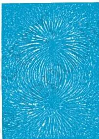
The pattern itself lets us plot magnetic field lines. Their four properties govern everything else in the chapter.
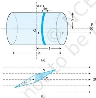
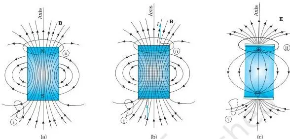
- (i) They form continuous closed loops. This is unlike the electric dipole, whose field lines begin on positive charge and end on negative charge, or escape to infinity (p. 137).
- (ii) The tangent at a point gives the direction of the net magnetic field B there.
- (iii) Crowding means strength. The more lines crossing unit area, the stronger B — in Fig 5.2(a) the field is larger around region (ii) than region (i).
- (iv) Lines never intersect. If they did, the direction of B would not be unique at the crossing point.
Misconception autopsy: why field lines are not “lines of force”
In electrostatics, a field line points along the force on a positive charge. In magnetism that idea fails: the magnetic force on a moving charge is \( q\mathbf{v} \times \mathbf{B} \), always perpendicular to B, never along the line (NCERT, p. 144). So the textbook deliberately drops the name “magnetic lines of force”.
The field line shows where a small compass needle aligns — not the direction a moving charge is pushed.
Bar magnet as an equivalent solenoid
Ampere’s hypothesis says all magnetic phenomena can be explained by circulating currents (p. 138). A bar magnet behaves like a solenoid of such currents, and its far axial field matches the solenoid’s exactly. Cutting a magnet in half is like cutting a solenoid — you get two smaller, weaker magnets, and the field lines stay continuous.
Since no cut ever isolates a single pole, magnetic monopoles do not exist (p. 136). You can test the analogy by moving a compass needle near a bar magnet and then near a current-carrying finite solenoid and watching identical deflections. For the solenoid field derivation, see our moving charges and magnetism notes.
Torque and Potential Energy of a Magnetic Dipole
In a uniform magnetic field, the net force on a dipole is zero — the two poles feel equal and opposite forces. Only a torque acts, tending to rotate the dipole into alignment with the field (NCERT, p. 139).
The torque is (p. 139):
\[ \boldsymbol{\tau} = \mathbf{m} \times \mathbf{B}, \qquad \tau = mB\sin\theta \]
where θ is the angle between m and B. Integrating \( \tau(\theta) \) against \( d\theta \) gives the magnetic potential energy:
\[ U_m = \int mB\sin\theta \, d\theta = -mB\cos\theta = -\mathbf{m}\cdot\mathbf{B} \]
Why the minus sign? The torque is a restoring torque — it does work against you when you rotate m away from B, so energy is lowest when the dipole aligns. The zero of energy is fixed at \( \theta = 90^\circ \) (needle perpendicular to the field). Then:
- θ = 0°: \( U_m = -mB \), the minimum — most stable position (parallel).
- θ = 180°: \( U_m = +mB \), the maximum — most unstable position (anti-parallel).
Units: torque in N m, energy in J (p. 139).
Axial and Equatorial Fields: The Electrostatic Analogy
The magnetic field of a short bar magnet at large distance can be written down from the electric dipole field by three replacements (NCERT, p. 140):
\[ \mathbf{E} \rightarrow \mathbf{B}, \qquad \mathbf{p} \rightarrow \mathbf{m}, \qquad \frac{1}{4\pi\varepsilon_0} \rightarrow \frac{\mu_0}{4\pi} \]
For a short magnet of size \( l \), at distance \( r \gg l \) from its midpoint:
\[ \text{Axial: } \mathbf{B}_A = \frac{\mu_0}{4\pi}\frac{2\mathbf{m}}{r^3} \qquad (\text{Eq. 5.5}) \]
\[ \text{Equatorial: } \mathbf{B}_E = -\frac{\mu_0}{4\pi}\frac{\mathbf{m}}{r^3} \qquad (\text{Eq. 5.4}) \]
The minus sign on the equator simply states that the field there points opposite to m. The axial equation (5.5) is the same as the equivalent-solenoid far field (Eq. 5.1, p. 138) — that identity is why the bar magnet and solenoid produce identical far fields.
Exam-friendly fact: at the same distance the axial magnitude is twice the equatorial magnitude: \( B_A = 2\,B_E \).
The dipole analogy (compact Table 5.1)
| Quantity | Electrostatics | Magnetism |
|---|---|---|
| Dipole moment | \( \mathbf{p} \) | \( \mathbf{m} \) |
| Equatorial field (short dipole) | \( -\frac{\mathbf{p}}{4\pi\varepsilon_0 r^3} \) | \( -\frac{\mu_0\mathbf{m}}{4\pi r^3} \) |
| Axial field (short dipole) | \( \frac{2\mathbf{p}}{4\pi\varepsilon_0 r^3} \) | \( \frac{\mu_0 2\mathbf{m}}{4\pi r^3} \) |
| Torque in external field | \( \mathbf{p} \times \mathbf{E} \) | \( \mathbf{m} \times \mathbf{B} \) |
| Potential energy | \( -\mathbf{p}\cdot\mathbf{E} \) | \( -\mathbf{m}\cdot\mathbf{B} \) |
Gauss’s Law of Magnetism: Why No Monopoles
Compare the two Gauss laws side by side (NCERT, p. 142):
\[ \text{Electrostatics: } \sum \mathbf{E}\cdot\Delta\mathbf{S} = \frac{q}{\varepsilon_0} \qquad \text{Magnetism: } \phi_B = \sum \mathbf{B}\cdot\Delta\mathbf{S} = 0 \]
Why is the magnetic side zero? Magnetic field lines are continuous closed loops, so every line that enters a closed surface also leaves it — there are no sources or sinks of B (p. 142). The simplest magnetic element is therefore a dipole or a current loop, never an isolated pole.
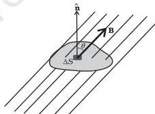
The “if monopoles existed” twist: Gauss’s law would become \( \oint \mathbf{B}\cdot\Delta\mathbf{S} = \mu_0 q_m \), where \( q_m \) is the magnetic charge enclosed (p. 144). This is a favourite conceptual question — one mark for the statement \( \oint \mathbf{B}\cdot\Delta\mathbf{S} = 0 \), one for the monopole modification.
Magnetisation, Magnetic Intensity and Susceptibility
This is the chain students find confusing — build it in order (NCERT, p. 145–146).
- Magnetisation — net magnetic moment per unit volume: \( \mathbf{M} = \frac{\mathbf{m}_{\text{net}}}{V} \), unit A m⁻¹ (Eq. 5.7).
- Empty solenoid field — \( \mathbf{B}_0 = \mu_0 n I \), unit T (Eq. 5.8); \( n \) = turns per metre.
- With a material core — the total field grows: \( \mathbf{B} = \mathbf{B}_0 + \mathbf{B}_m \), with \( \mathbf{B}_m = \mu_0 \mathbf{M} \) (Eqs. 5.9, 5.10).
- Magnetic intensity — \( \mathbf{H} = \frac{\mathbf{B}}{\mu_0} – \mathbf{M} \), unit A m⁻¹ (Eq. 5.11), which rearranges to \( \mathbf{B} = \mu_0(\mathbf{H} + \mathbf{M}) \) (Eq. 5.12).
- Linear materials — \( \mathbf{M} = \chi\mathbf{H} \), with χ the dimensionless magnetic susceptibility (Eq. 5.13).
- One tidy line — \( \mathbf{B} = \mu_0(1+\chi)\mathbf{H} = \mu_0\mu_r\mathbf{H} = \mu\mathbf{H} \), where \( \mu_r = 1+\chi \) and \( \mu = \mu_0\mu_r \) (Eqs. 5.14, 5.15).
The physical split to remember: H carries the external contribution (currents in the solenoid); M carries the material’s response. Only one of \( \chi \), \( \mu_r \), \( \mu \) is independent — given any one, the other two follow (p. 146).
Diamagnetic, Paramagnetic and Ferromagnetic Materials Compared
Susceptibility alone sorts the materials. Table 5.2 gives the ranges (NCERT, p. 147), where \( \varepsilon \) is a small positive number:
| Property | Diamagnetic | Paramagnetic | Ferromagnetic |
|---|---|---|---|
| Susceptibility χ | \( -1 \le \chi \lt 0 \) | \( 0 \lt \chi \lt \varepsilon \) | \( \chi \gg 1 \) |
| Relative permeability μ_r | \( 0 \le \mu_r \lt 1 \) | \( 1 \lt \mu_r \lt 1+\varepsilon \) | \( \mu_r \gg 1 \) |
| Permeability μ | \( \mu \lt \mu_0 \) | \( \mu \gt \mu_0 \) | \( \mu \gg \mu_0 \) |
The comparison below is the table to recall in the exam hall.
| Feature | Diamagnetic | Paramagnetic | Ferromagnetic |
|---|---|---|---|
| Behaviour in a non-uniform field | Repelled — moves from stronger to weaker field | Weakly attracted — moves from weaker to stronger field | Strongly attracted |
| Origin | Zero net atomic moment; applied field induces an opposite moment (Lenz’s law) | Permanent atomic dipoles, randomised by thermal motion, aligned by the field | Spontaneous alignment of atoms over macroscopic domains |
| Examples | Bismuth, copper, lead, silicon, water, sodium chloride, nitrogen | Aluminium, sodium, calcium, oxygen, copper chloride | Iron, cobalt, nickel, gadolinium |
| Strength of effect | Field slightly reduced (~1 part in 10⁵) | Field slightly enhanced (~1 part in 10⁵) | Field highly concentrated; μ_r > 1000 |
| Special case | Superconductors: perfect diamagnets (χ = −1) | — | Becomes paramagnetic at high temperature |
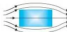
Why diamagnetics are repelled (p. 147): orbiting electrons act as current loops with orbital magnetic moments. In a diamagnetic material the net atomic moment is zero. An applied field induces extra currents (Lenz’s law — studied in our electromagnetic induction notes) that slow electrons aligned with the field and speed up those opposed, producing a net moment opposite to B.
Opposite moment, negative χ, repulsion.
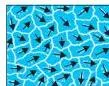
Domains are the key to ferromagnetism (p. 149): atoms interact so strongly that they align spontaneously over a macroscopic region called a domain — typically about 1 mm across, containing about 10¹¹ atoms. An applied field makes the aligned domains grow until they merge into one giant domain.
- Hard ferromagnets (Alnico, lodestone) retain magnetisation after the field is removed — they make permanent magnets and compass needles.
- Soft ferromagnets (soft iron) lose magnetisation when the field is removed.
- Temperature: at high enough temperature a ferromagnet becomes a paramagnet as the domain structure disintegrates (p. 149).
Memory device for the sign of χ — “Diamonds Dive (negative), Parrots Persist a little (small positive), Ferocious Fields Flood (huge positive).”
Definitions Table: Terms You Must Know
| Term | Meaning | Example / unit |
|---|---|---|
| Magnetic moment m | Strength of a magnetic dipole | A m²; for a solenoid \( m = NIA \) |
| Magnetic flux φ_B | \( \mathbf{B}\cdot\Delta\mathbf{S} \) through a surface | Weber (Wb); 1 Wb = 1 T m² |
| Magnetisation M | Net magnetic moment per unit volume | A m⁻¹ |
| Magnetic intensity H | External-field contribution; \( H = B/\mu_0 – M \) | A m⁻¹; \( H = nI \) in a solenoid |
| Magnetic susceptibility χ | How a material responds to H; \( M = \chi H \) | Dimensionless; negative dia, small positive para, large ferro |
| Relative permeability μ_r | \( 1 + \chi \) | Dimensionless |
| Permeability μ | \( \mu_0\mu_r \) | T m A⁻¹ |
| Domain | Macroscopic region of aligned atomic moments in a ferromagnet | ~1 mm, ~10¹¹ atoms |
| Magnetic monopole | Isolated magnetic pole | Does not exist |
| Meissner effect | Perfect diamagnetism: total expulsion of field in a superconductor | χ = −1, μ_r = 0 |
| Hard / soft ferromagnet | Retains / loses magnetisation after field removed | Alnico, lodestone / soft iron |
| Magnetising current I_m | Extra current giving the same B without a core | \( I_m = (\mu_r – 1)I \) |
Formula Sheet: All Equations with Units
Every equation from the chapter in one table (NCERT, p. 138–151). Constants: \( \frac{\mu_0}{4\pi} = 10^{-7} \ \) T m A⁻¹, \( 1 \ \)T \( = 10^4 \) G, \( 1 \) Wb \( = 1 \) T m².
| Formula | Meaning | Units / remarks |
|---|---|---|
| \( \boldsymbol{\tau} = \mathbf{m}\times\mathbf{B} \) | Torque on a dipole in a uniform field | N m; \( \theta \) is the angle between m and B |
| \( \tau = mB\sin\theta \) | Magnitude of that torque | N m |
| \( U_m = -\mathbf{m}\cdot\mathbf{B} = -mB\cos\theta \) | Magnetic potential energy | J; zero at 90°, min −mB at 0°, max +mB at 180° |
| \( B_A = \frac{\mu_0}{4\pi}\frac{2m}{r^3} \) | Far axial field of a short magnet | T; valid for \( r \gg l \) |
| \( B_E = -\frac{\mu_0}{4\pi}\frac{m}{r^3} \) | Far equatorial field of a short magnet | T; \( |B_A| = 2|B_E| \) |
| \( \phi_B = \sum \mathbf{B}\cdot\Delta\mathbf{S} = 0 \) | Gauss’s law of magnetism | Wb |
| \( \mathbf{M} = \mathbf{m}_{\text{net}}/V \) | Magnetisation | A m⁻¹ |
| \( B_0 = \mu_0 n I \) | Field inside an empty solenoid | T |
| \( \mathbf{B} = \mu_0(\mathbf{H}+\mathbf{M}) \) | Total field inside a material | T |
| \( H = B/\mu_0 – M \), \( H = nI \) | Magnetic intensity | A m⁻¹ |
| \( M = \chi H \) | Linear material response | A m⁻¹; \( \chi \) dimensionless |
| \( B = \mu_0(1+\chi)H = \mu_0\mu_r H = \mu H \) | Field via permeability | T; only one of χ, μ_r, μ is independent |
| \( \mu = \mu_0\mu_r = \mu_0(1+\chi) \) | Magnetic permeability | T m A⁻¹ |
You can open the official NCERT Class 12 Physics Part I chapter 5 PDF to verify any formula or figure directly against the source.
Worked Examples: Numerical Problems Step by Step
Worked Example 1: Torque and potential energy of a magnetic needle
Method: substitute directly into \( \tau = mB\sin\theta \) and \( U = -mB\cos\theta \), keeping the angle between m and B (Eqs. 5.2, 5.3, NCERT p. 139).
Given: a needle of magnetic moment \( m = 0.60 \ \)A m² in a uniform field \( B = 0.35 \ \)T, making \( \theta = 60^\circ \) with the field.
Step 1: Torque magnitude.
\[ \tau = mB\sin\theta = 0.60 \times 0.35 \times \sin 60^\circ = 0.21 \times 0.866 \approx 0.18 \ \text{N m} \]
Step 2: Potential energy at 60°.
\[ U = -mB\cos 60^\circ = -0.21 \times 0.5 = -0.105 \ \text{J} \]
Step 3: The limiting orientations — at \( \theta = 0^\circ \), \( U = -mB = -0.21 \) J (stable equilibrium); at \( \theta = 180^\circ \), \( U = +mB = +0.21 \) J (unstable equilibrium).
Final answer: \( \tau \approx 0.18 \) N m, \( U \approx -0.105 \) J; stable at 0° with −0.21 J, unstable at 180° with +0.21 J.
Worked Example 2: Axial and equatorial field of a short bar magnet
Method: use Eqs. 5.5 and 5.4 with \( \mu_0/4\pi = 10^{-7} \ \)T m A⁻¹, valid because \( r \gg l \) (NCERT p. 140).
Given: \( m = 2.0 \) A m², \( r = 0.20 \) m measured from the magnet’s centre.
- Step 1: Compute \( r^3 = (0.20)^3 = 8.0 \times 10^{-3} \ \)m³.
- Step 2: Axial field on the axis.
\[ B_A = 10^{-7} \times \frac{2 \times 2.0}{(0.20)^3} = 10^{-7} \times \frac{4.0}{8.0 \times 10^{-3}} = 10^{-7} \times 500 = 5.0 \times 10^{-5} \ \text{T} \]
Step 3: Equatorial field on the normal bisector (magnitude):
\[ B_E = 10^{-7} \times \frac{2.0}{(0.20)^3} = 10^{-7} \times 250 = 2.5 \times 10^{-5} \ \text{T} \]
Step 4: Check the ratio: \( B_A / B_E = 2.0 \) — the axial field is double the equatorial, directed along \( \mathbf{m} \) on the axis and opposite to \( \mathbf{m} \) on the equator.
Final answer: \( B_A = 5.0 \times 10^{-5} \) T along the axis; \( B_E = 2.5 \times 10^{-5} \) T opposite to m on the equator.
Worked Example 3: Solenoid with a material core — H, B, M and magnetising current
Method: follow the Example 5.5 pattern (NCERT p. 146): H first, then B, then M, then the magnetising current.
Given: \( n = 1500 \) turns/m, \( I = 1.5 \) A, core with \( \mu_r = 200 \).
Step 1: Magnetic intensity depends only on the solenoid, not the core: \( H = nI \).
\[ H = 1500 \times 1.5 = 2250 \ \text{A/m} \]
Step 2: Total field \( B = \mu_r\mu_0 H \).
\[ B = 200 \times 4\pi \times 10^{-7} \times 2250 \approx 200 \times 2.83 \times 10^{-3} \approx 0.57 \ \text{T} \]
Step 3: Magnetisation \( M = (\mu_r – 1)H \).
\[ M = 199 \times 2250 \approx 4.5 \times 10^5 \ \text{A/m} \]
Step 4: Magnetising current \( I_m = (\mu_r – 1)I \).
\[ I_m = 199 \times 1.5 = 298.5 \ \text{A} \]
Step 5 (check): \( I + I_m = 1.5 + 298.5 = 300 \) A and \( \mu_r I = 200 \times 1.5 = 300 \) A — the two agree, confirming the calculation.
Final answer: \( H = 2250 \) A/m, \( B \approx 0.57 \) T, \( M \approx 4.5 \times 10^5 \) A/m, \( I_m = 298.5 \) A; check \( I + I_m = \mu_r I \).
Common Mistakes Students Make in Magnetism and Matter
| Students write… | Correct is… | How to check your answer |
|---|---|---|
| Field lines start at N and end at S | Lines are continuous closed loops; inside the magnet they run from S to N | Trace any line — it must return to its starting point (p. 137) |
| Cutting a magnet isolates a pole | Each half is a weaker two-pole magnet; monopoles do not exist | Suspending a half still aligns it N–S (p. 136, 138) |
| χ is positive for diamagnetics | χ negative for dia, small positive for para, large positive for ferro | For dia, \( M = \chi H \) must put M opposite to H (p. 146–147) |
| μ_r = 0 for all diamagnetics | Only superconductors have exactly μ_r = 0 (χ = −1); ordinary dia have \( 0 \le \mu_r \lt 1 \) | Use \( \mu_r = 1 + \chi \) (p. 147) |
| Diamagnetics are attracted | They are repelled, moving from stronger to weaker field | Negative χ means the induced moment opposes the field (p. 147) |
| B and H are the same | \( B = \mu_0(H+M) \); H is external, M is material, B is total | Units: B in tesla, H and M in A m⁻¹ (p. 145–146) |
| Zero potential energy at θ = 0° | Zero is fixed at θ = 90°; U is minimum (−mB) at 0° and maximum (+mB) at 180° | Substitute into \( U = -mB\cos\theta \) (p. 139) |
| Axial field equals equatorial field | At the same distance the axial magnitude is twice the equatorial | Compare \( B_A = (\mu_0/4\pi)(2m/r^3) \) with \( B_E \) (p. 140) |
Exam Notes: How This Chapter Is Tested
Patterns below come from the textbook’s own exercises, stated with the step that earns the mark. No prediction — just what the book itself asks.
- Torque and energy numericals (Exercises 5.1, 5.2, 5.5): direct substitution into \( \tau = mB\sin\theta \) and \( U = -mB\cos\theta \), plus work done \( = \) change in U when rotating between orientations. The credit step: explicitly stating that \( \theta = 0^\circ \) is stable and \( \theta = 180^\circ \) is unstable. Work is quoted in joules; torque in N m.
- Solenoid-as-magnet numericals (Exercises 5.3, 5.4, 5.6): first find \( m = NIA \), then the torque on that dipole \( \tau = mB\sin\theta \). Keeping the turns and area distinct earns the mark.
- Field numericals (Exercise 5.7): convert 10 cm into 0.10 m before cubing, use \( \mu_0/4\pi = 10^{-7} \), and report the relation “axial = 2 × equatorial” with direction (on the axis along m, on the equator opposite).
- Core numericals (Example 5.5 pattern): fixed order H → B → M → I_m. The elegant check \( I + I_m = \mu_r I \) is a quick way to verify.
- Conceptual favourites: Example 5.1 (cutting magnets, nail attraction, why a toroid has no poles), Example 5.3 (wrong field-line diagrams), Example 5.4 (monopoles modify Gauss’s law; field lines are not lines of force), and the units table (\( 1 \) T \( = 10^4 \) G, \( 1 \) Wb \( = 1 \) T m²).
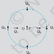
Figure 5.4 reasoning (Example 5.2, p. 141): equilibrium is stable when \( \mathbf{m}_Q \) is parallel to the field of P, and unstable when anti-parallel. Q₃ and Q₆ are stable, Q₄ and Q₅ unstable, and Q₆ has the lowest potential energy because m aligns fully with the field.
Reading the Field Line Diagrams Like an Examiner
The textbook’s Fig 5.6 (Example 5.3, p. 143) shows seven field-line sketches, several deliberately wrong. Auditing them with the four field-line rules is the quickest way to internalise the closed-loop property.
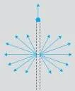
- (c) Correct — magnetic lines fully confined in a toroid; each closed loop encloses a current-carrying region.
- (e) Correct — bar magnet lines. Inside the magnet lines run from S to N, and the net flux around each pole is zero.
- (a) Wrong — lines emanate from a point, implying a source of B. That sketch is the electric field of a long positively charged wire.
- (b) Wrong — two defects: lines cross (direction ambiguous at the intersection) and a static magnetic loop forms around empty space, but a closed static magnetic loop must enclose a current.
- (d) Wrong — solenoid ends cannot be straight and confined; that would violate Ampere’s law. Lines must curve out at both ends and close.
- (f) Wrong — all lines leave one plate, so net flux through a surface around the plate is non-zero — impossible for magnetism. It actually shows the electrostatic field between charged plates.
- (g) Wrong — pole pieces cannot give perfectly straight lines at the ends; some fringing is unavoidable (also true for electric field lines).
Magnetism and Matter Class 12 Notes: One-Page Revision Summary
- A bar magnet is a magnetic dipole; poles always come in pairs and monopoles do not exist (p. 136).
- In a uniform field, net force is zero; only torque acts, \( \tau = mB\sin\theta \) (p. 139).
- Potential energy \( U = -mB\cos\theta \), zero at 90°, minimum −mB at 0° (stable), maximum +mB at 180° (unstable) (p. 139).
- Far axial field \( (\mu_0/4\pi)(2m/r^3) \), far equatorial \( -(\mu_0/4\pi)(m/r^3) \); axial magnitude is double the equatorial (p. 140).
- Gauss’s law of magnetism: net flux through any closed surface is zero; no sources or sinks of B (p. 142).
- \( M = m_{\text{net}}/V \); total field \( B = \mu_0(H + M) \); H is the external contribution, M the material’s response (p. 145).
- \( M = \chi H \), \( B = \mu_0\mu_r H = \mu H \), \( \mu_r = 1 + \chi \); only one of χ, μ_r, μ is independent (p. 146).
- Dia: χ negative, repelled; para: χ small positive, weakly attracted; ferro: χ ≫ 1, strongly attracted via domains (p. 147–149).
- Hard ferromagnets (Alnico, lodestone) retain magnetisation and make permanent magnets; soft iron loses it (p. 149).
- Superconductors are perfect diamagnets (Meissner effect, χ = −1, μ_r = 0); a ferromagnet becomes paramagnetic at high temperature as domains disintegrate (p. 147–149).
For the full set of chapter resources, browse all Class 12 notes or the complete CBSE notes library.
FAQs on Magnetism and Matter for Class 12
Why do magnetic field lines form closed loops while electric field lines do not?
Because isolated magnetic poles do not exist. Magnetic field lines are continuous closed loops, so any line entering a closed surface also leaves it — net flux is zero (NCERT, p. 142). Electric field lines begin on positive charge and end on negative charge, or escape to infinity, which is why an electric dipole’s lines do not close (p. 137).
Can we isolate a north pole by cutting a bar magnet into two pieces?
No. Cutting a bar magnet — across its length or along it — gives two smaller magnets, each with a north and a south pole (p. 139). The poles stay paired because a magnet behaves like a solenoid of circulating currents, and no cut breaks a solenoid into single poles (p. 138).
Why is a diamagnetic substance repelled by a magnet?
Because it develops a net magnetic moment opposite to the applied field. Orbiting electrons respond through induced currents (Lenz’s law) that slow electrons aligned with the field and speed up those opposed, producing the opposite moment (p. 147). Since M and H point opposite ways, χ is negative and the substance is repelled.
What is the difference between magnetic intensity H, magnetisation M and magnetic field B?
H is the external contribution to the field (currents in the solenoid); M is the material’s response, its net magnetic moment per unit volume (p. 145–146). They combine as \( B = \mu_0(H + M) \): B is the total field inside the material. H and M share the unit A m⁻¹, while B is in tesla (p. 151).
Why does an iron nail experience a force but a compass needle only a torque in a uniform magnetic field?
In a uniform field the net force on a dipole is zero, so a needle feels only the torque \( \tau = \mathbf{m} \times \mathbf{B} \) (p. 139).
The nail sits in the non-uniform field of the bar magnet, which induces a magnetic moment in it, and a non-uniform field exerts a net force on that induced moment — an attractive one, because the induced near pole is of opposite type (p. 139–140).
What is the Meissner effect and what are the values of χ and μ_r for a superconductor?
The Meissner effect is perfect diamagnetism: a superconductor completely expels magnetic field lines from its interior (p. 147–148). For a superconductor χ = −1 and μ_r = 0, so μ = 0 and the field inside is exactly zero (p. 151). This is why a superconductor repels a magnet and is itself repelled.
What is the magnetising current of a solenoid with a core and how is it calculated?
It is the extra current that would produce the same B in the solenoid without the core (p. 146). From \( B = \mu_r\mu_0 n(I + I_m) \), you get \( I_m = (\mu_r – 1)I \). In Example 5.5 (n = 1000 turns/m, I = 2 A, μ_r = 400) the magnetising current is 794 A (p. 146).
Reference: NCERT Class 12 Physics Part I textbook, chapter Magnetism and Matter.
Explore Class 12 Physics Notes
More for this chapter:
Class 12 Physics on LearnCBSE:
Related chapters: