
Atoms class 12 notes — this page compresses the whole chapter into a revision-ready form: Thomson’s plum pudding model, the Geiger–Marsden experiment that produced Rutherford’s nuclear model, Bohr’s three postulates and hydrogen’s energy levels, line spectra, and de Broglie’s standing-wave explanation of quantisation.
Everything is condensed — definitions, formulas with symbol meanings, worked examples using original numbers, and exam pointers — so you can revise the chapter alone, even the night before a test.
Each formula and figure below is tied to the page of the NCERT Class 12 Physics Part II textbook (chapter “Atoms”) where it appears, so you can cross-check quickly. Use the jump links to reach any topic directly.
Related material: Class 12 Physics notes for every chapter, all Class 12 notes, and the full CBSE notes library.
The Race to Model the Atom: Thomson to Bohr
By the late 1800s, experiments on electric discharge through gases showed that all atoms carry identical negative particles — electrons — yet atoms as a whole are electrically neutral. So every atom must also hold positive charge. The open question was how that charge and the electrons are arranged (NCERT, p. 1).
Three models answered the question in turn, each fixing a fatal flaw in the one before:
- Thomson (1898): the atom is a spherical cloud of positive charge with electrons embedded in it, “like seeds in a watermelon” — the plum pudding model. It guessed at the arrangement but said nothing about why atoms emit discrete wavelengths (p. 1).
- Rutherford (1911): nearly all the mass and all the positive charge sit in a tiny nucleus, with electrons orbiting like planets round the sun. It came from the alpha-scattering data, but could not explain why atoms are stable or why they give line spectra (p. 1).
- Bohr (1913): kept the nuclear picture but added three quantum postulates, so electrons occupy only certain stable orbits and emit light at discrete frequencies. It explains hydrogen’s spectrum, though only for single-electron atoms (p. 8–10).
The progression matters for exams: each model’s failure is as important as its success. A comparison table is the quickest way to hold all three together.
| Feature | Thomson’s model | Rutherford’s model | Bohr’s model |
|---|---|---|---|
| Positive charge | Spread uniformly through the atom | Concentrated in a tiny central nucleus | Same nucleus as Rutherford |
| Electron arrangement | Embedded like seeds in a watermelon | Revolving in any orbit, like planets | Only in fixed stationary orbits |
| Stability | Unstable electrostatically | Classically unstable — electron must radiate and collapse | Stable by postulate — no radiation in stationary orbits |
| Spectra explained | None | Predicts a continuous spectrum only | Explains discrete line spectra of hydrogen |
| Main failure | Wrong charge arrangement | Atom collapses; wrong spectrum | Only hydrogenic atoms; no line intensities |
Geiger–Marsden Experiment: What the Data Said
In 1911, Geiger and Marsden — working on Rutherford’s suggestion — fired a beam of 5.5 MeV alpha particles (helium nuclei, charge \( 2e \)) from a \( ^{214}_{83}\text{Bi} \) source at a thin gold foil. Lead bricks collimated the beam into a narrow stream, and a rotatable zinc-sulphide screen detected each scattered particle as a tiny flash (scintillation) (NCERT, p. 2–3).
The foil was only \( 2.1 \times 10^{-7}\ \text{m} \) thick.
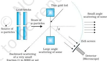
Two statistics from the data shaped everything that followed (p. 3):
- only about 0.14% of the alphas scattered by more than 1°;
- only about 1 in 8000 deflected by more than 90° — a few even bounced back.
Rutherford’s reasoning: to throw an alpha backwards, the target must exert a huge repulsive force, and that is only possible if the atom’s positive charge and most of its mass are packed into a tiny central region. The deflected particle almost meets that charge head-on without penetrating it.
The data matched a model of a small, dense, positively charged nucleus so well that Rutherford is credited with discovering the nucleus (p. 3).
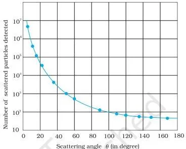
The measured nucleus size came out about \( 10^{-15} \) to \( 10^{-14}\ \text{m} \), while the atom is about \( 10^{-10}\ \text{m} \) — 10,000 to 100,000 times larger. In other words, an atom is mostly empty space, which is exactly why most alphas pass straight through (p. 3).
The force deflecting an alpha at distance \( r \) from a nucleus of atomic number \( Z \) is Coulomb repulsion (Eq. 12.1, p. 5):
\[ F = \frac{1}{4\pi\epsilon_0}\frac{(2e)(Ze)}{r^2} \]
For gold, \( Z = 79 \). The gold nucleus, being about 50 times heavier than an alpha, stays essentially fixed during the encounter. This same force controls the alpha’s path, and its size sets the impact parameter and the distance of closest approach below.
Impact Parameter and the Scattering Angle
The impact parameter \( b \) is the perpendicular distance of the alpha’s initial velocity vector from the centre of the nucleus (Fig. 12.4, NCERT, p. 5). A beam contains alphas with many impact parameters, so they scatter in all directions with different probabilities.
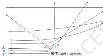
The link between \( b \) and the scattering angle \( \theta \) is the core idea:
- Small \( b \) (near head-on) → strong repulsion → large deflection; at the minimum \( b \), the alpha rebounds back (\( \theta \approx \pi \)).
- Large \( b \) (a grazing pass) → the alpha goes nearly undeviated (\( \theta \approx 0 \)).
Because so few alphas rebound, head-on collisions must be rare — and that rarity is why Rutherford could place an upper limit on the nuclear size (p. 5).
Distance of Closest Approach
For a head-on collision, the alpha slows as it climbs the Coulomb repulsion hill until it momentarily stops, then reverses. At that turning point its kinetic energy \( K \) has fully converted into electric potential energy. Energy conservation gives (NCERT, p. 5–6):
\[ K = \frac{2Ze^2}{4\pi\epsilon_0 d} \quad \Rightarrow \quad d = \frac{2Ze^2}{4\pi\epsilon_0 K} \]
Here \( e \) is the electronic charge, \( 1/4\pi\epsilon_0 = 9.0 \times 10^9\ \text{N m}^2/\text{C}^2 \), and \( Z \) is the target’s atomic number. A 7.7 MeV alpha on gold (\( Z = 79 \)) gives \( d = 3.0 \times 10^{-14}\ \text{m} = 30\ \text{fm} \), whereas the actual gold nucleus radius is only about 6 fm (p. 6).
The crucial exam point: \( d \) is an upper limit on the nuclear radius, not the radius itself. The alpha reverses before it ever touches the nucleus — it stops at the edge of an imaginary sphere of radius \( d \) centred on the nucleus.
Classical Physics Cannot Explain the Atom
Rutherford’s model treated the electron like a planet, but the analogy fails for two reasons (NCERT, p. 8):
- Collapse: an electron moving in a circle is constantly accelerating (centripetal acceleration \( v^2/r \)). Classical electrodynamics says any accelerating charge radiates energy. The electron would lose energy, spiral inward, and crash into the nucleus — atoms could not be stable.
- Wrong spectrum: as the electron spirals, its orbital frequency changes continuously, so the emitted light would form a continuous spectrum. Real atoms emit discrete line spectra.
A common trap: students argue the electron keeps a constant speed, so it cannot radiate. Reject that — constant speed does not mean zero acceleration; the direction keeps changing, and that is what forces radiation.
The orbit maths that exposes the problem (p. 6–7): balancing electric force with centripetal force, \[ \frac{1}{4\pi\epsilon_0}\frac{e^2}{r^2} = \frac{mv^2}{r} \]
gives the orbit radius–velocity relation \( r = e^2/(4\pi\epsilon_0 m v^2) \) (Eq. 12.3), and the total energy \[ E = K + U = \frac{e^2}{8\pi\epsilon_0 r} – \frac{e^2}{4\pi\epsilon_0 r} = -\frac{e^2}{8\pi\epsilon_0 r} \]
The negative sign means the electron is bound: you must supply energy to free it. If \( E \) were positive, the electron would not follow a closed orbit at all (p. 7).
Bohr’s Three Postulates
In 1913 Niels Bohr added early quantum ideas to Rutherford’s nucleus. His model rests on three postulates (NCERT, p. 8–10):
- Stationary orbits: the electron can revolve in certain stable orbits without radiating, despite the classical prediction. Each stable state has a definite total energy — these are the stationary states of the atom.
- Quantised angular momentum: the electron orbits only where its angular momentum is an integral multiple of \( h/2\pi \): \( L = nh/2\pi \) (Eq. 12.5), with \( h = 6.6 \times 10^{-34}\ \text{J s} \) and \( n = 1, 2, 3, \dots \).
- Transitions: when the electron jumps from a higher to a lower stationary state, a photon is emitted whose energy equals the difference: \( h\nu = E_i – E_f \) (Eq. 12.6), where \( E_i \gt E_f \).
Memory device — SAT: Stationary orbits, Angular momentum quantised, Transition emits a photon.
Applying the quantisation condition to the orbit equations yields the radius of the \( n \)-th orbit (Eq. 12.7):
\[ r_n = \left(\frac{n^2}{m}\right)\left(\frac{h}{2\pi}\right)^2 \frac{4\pi\epsilon_0}{e^2} \]
and the corresponding energy (Eqs. 12.8–12.10):
\[ E_n = -\frac{me^4}{8n^2\epsilon_0^2 h^2} = -\frac{2.18 \times 10^{-18}}{n^2}\ \text{J} = -\frac{13.6}{n^2}\ \text{eV} \]
Because \( n \) is a whole number, both the radii and the energies come out in discrete steps — that discreteness is what produces discrete spectral lines.
Energy Levels and Ionisation Energy of Hydrogen
The energy-level diagram (Fig. 12.7, NCERT, p. 11) plots \( E_n \) against \( n \) and is worth learning precisely:
- Ground state \( n = 1 \): \( E = -13.6\ \text{eV} \) — the lowest (most negative) energy, smallest orbit.
- First excited state \( n = 2 \): \( E = -3.40\ \text{eV} \); second excited \( n = 3 \): \( E = -1.51\ \text{eV} \).
- Levels crowd closer together as \( n \) grows; \( n = \infty \) corresponds to \( E = 0\ \text{eV} \), the electron removed and at rest.
- Above \( E = 0\ \text{eV} \) lies a continuum of free-electron states.
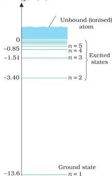
Two energies you will be asked for repeatedly (p. 11):
- Ionisation energy: 13.6 eV, the minimum energy to free the ground-state electron.
- First excitation energy: \( E_2 – E_1 = -3.40 – (-13.6) = 10.2\ \text{eV} \), to raise the atom from \( n = 1 \) to \( n = 2 \).
Common trap: the bound electron has negative total energy, yet 0 eV means the electron is free, not at ground state. The ground state is the most negative point on the diagram.
Hydrogen Line Spectra as a Fingerprint
An excited rarefied gas emits an emission line spectrum — bright lines on a dark background — because individual atoms, not interacting neighbours, radiate (NCERT, p. 7).
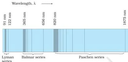
When white light passes through the same gas, the transmitted spectrum shows dark lines at exactly the wavelengths the gas would emit — the absorption spectrum of that material (p. 7). Emission and absorption lines are two views of the same allowed energy jumps.
The transition rule (Eq. 12.11, p. 11):
\[ h\nu_{if} = E_{n_i} – E_{n_f}, \quad n_f \lt n_i \]
Since both \( n_i \) and \( n_f \) are integers, the emitted frequencies are forced to discrete values — that is the physical reason spectra are not continuous.
Real-life fingerprinting: an element’s line spectrum is unique, a “fingerprint” for identifying a gas (p. 7). This is how astronomers identify elements in starlight — matching the dark absorption lines in the star’s spectrum against known laboratory lines — and it is why neon signs glow red and mercury vapour lamps emit their characteristic blue-green light.
The historical clue came early: in 1885 Balmer fitted a simple empirical formula to a group of hydrogen lines (p. 1), and Bohr’s model later explained them from first principles.
de Broglie’s Standing-Wave Explanation
Bohr’s second postulate — quantised angular momentum — looks arbitrary. In 1923 Louis de Broglie explained why it must hold (NCERT, p. 12–13). From Chapter 11’s idea, the electron is also a wave with wavelength \( \lambda = h/mv \).
Like a plucked string, where only standing waves with nodes at the ends survive, an electron on a circular orbit keeps only the waves that close on themselves — whole numbers of wavelengths fitting the circumference:
\[ 2\pi r_n = n\lambda, \quad n = 1, 2, 3, \dots \]
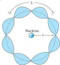
Substitute \( \lambda = h/(mv_n) \):
\[ 2\pi r_n = \frac{nh}{mv_n} \quad \Rightarrow \quad m v_n r_n = \frac{nh}{2\pi} \]
That is exactly Bohr’s quantisation condition. So the angular-momentum rule is not imposed by hand — it follows from the wave nature of the electron: only resonant standing waves can persist. The waveforms that do not close on themselves interfere destructively and die out instantly.
Your Dual Nature of Radiation and Matter notes carry the experimental proof (Davisson–Germer) that electrons really are waves.
Key Terms at a Glance
| Term | Meaning | Example from the chapter |
|---|---|---|
| Impact parameter | Perpendicular distance of the alpha’s initial velocity vector from the nucleus centre | Small \( b \) → large deflection (p. 5) |
| Distance of closest approach | Centre-to-centre distance where a head-on alpha momentarily stops and reverses | Gold with 7.7 MeV alphas: \( 3.0 \times 10^{-14}\ \text{m} \) (p. 6) |
| Stationary state | A stable orbit in which the electron radiates no energy | Postulate 1 of Bohr’s model (p. 8) |
| Ground state | Lowest-energy state, smallest orbit, \( n = 1 \) | \( E_1 = -13.6\ \text{eV} \) (p. 11) |
| Excited state | Any higher-energy state, \( n \gt 1 \) | \( E_2 = -3.40\ \text{eV} \) (p. 11) |
| Ionisation energy | Minimum energy to free the ground-state electron | 13.6 eV for hydrogen (p. 11) |
| Principal quantum number \( n \) | Integer labelling the stationary states in ascending energy | \( n = 1, 2, 3, \dots \) (p. 11) |
| Emission / line spectrum | Bright lines on a dark background from excited atoms | Hydrogen lines, Fig. 12.5 (p. 7) |
| Absorption spectrum | Dark lines where a gas absorbs the same wavelengths it emits | White light through a gas (p. 7) |
| Bohr radius \( a_0 \) | Radius of the innermost orbit, \( n = 1 \) | \( 5.3 \times 10^{-11}\ \text{m} \) (p. 6) |
| Hydrogenic atom | A nucleus \( +Ze \) with a single electron | H, \( \text{He}^+ \), \( \text{Li}^{2+} \) (p. 13) |
Formula Sheet: What the Board Exam Expects
| Quantity | Formula | Symbol meanings | Units |
|---|---|---|---|
| Coulomb force on an alpha (12.1) | \( F = \frac{1}{4\pi\epsilon_0}\frac{(2e)(Ze)}{r^2} \) | \( 2e \) alpha charge, \( Ze \) nucleus charge, \( r \) separation | N |
| Orbit balance (12.2–12.3) | \( \frac{1}{4\pi\epsilon_0}\frac{e^2}{r^2} = \frac{mv^2}{r} \), \( r = \frac{e^2}{4\pi\epsilon_0 m v^2} \) | \( m \) electron mass, \( v \) orbital speed | m |
| Energies in orbit (12.4) | \( K = \frac{e^2}{8\pi\epsilon_0 r} \), \( U = -\frac{e^2}{4\pi\epsilon_0 r} \), \( E = -\frac{e^2}{8\pi\epsilon_0 r} \) | \( K \) kinetic, \( U \) potential, \( E \) total energy | J |
| Quantised angular momentum (12.5) | \( L = \frac{nh}{2\pi} \) | \( n \) principal quantum number, \( h \) Planck constant | \( \text{J s} \) |
| Photon energy (12.6) | \( h\nu = E_i – E_f \) | \( E_i, E_f \) initial/final state energies | eV or J |
| Bohr orbit radius (12.7) | \( r_n = \left(\frac{n^2}{m}\right)\left(\frac{h}{2\pi}\right)^2 \frac{4\pi\epsilon_0}{e^2} \) | \( r_n = n^2 a_0 \), \( a_0 = 5.3 \times 10^{-11}\ \text{m} \) | m |
| Energy levels (12.8–12.10) | \( E_n = -\frac{me^4}{8n^2\epsilon_0^2 h^2} = -\frac{13.6}{n^2}\ \text{eV} \) | \( m, e, \epsilon_0, h \) as above | eV |
| Transition frequency (12.11) | \( h\nu_{if} = E_{n_i} – E_{n_f} \) | \( n_i \) initial, \( n_f \) final (lower) level | eV or J |
| Standing-wave condition (12.12) | \( 2\pi r_n = n\lambda \) | \( \lambda = h/(mv_n) \) de Broglie wavelength | m |
| Distance of closest approach | \( d = \frac{2Ze^2}{4\pi\epsilon_0 K} \) | \( K \) alpha kinetic energy, \( Z \) target number | m |
Every equation above is printed in the NCERT text; the official NCERT website hosts the free PDF of Physics Part II (chapter “Atoms”) if you want to verify a symbol or a page.
Worked Examples with Fresh Numbers
Example A: Distance of closest approach for a copper target
Method: Energy conservation — at the turning point the alpha’s kinetic energy equals the electric potential energy.
Step 1: Convert kinetic energy to joules.
\( K = 4.0\ \text{MeV} = 4.0 \times 1.6 \times 10^{-13}\ \text{J} = 6.4 \times 10^{-13}\ \text{J} \).
Step 2: Write the formula with \( Z = 29 \) for copper, \( e = 1.6 \times 10^{-19}\ \text{C} \), \( 1/4\pi\epsilon_0 = 9.0 \times 10^9\ \text{N m}^2/\text{C}^2 \).
\[ d = \frac{2(9.0 \times 10^9)(29)(1.6 \times 10^{-19})^2}{6.4 \times 10^{-13}} = \frac{1.34 \times 10^{-26}\ \text{J}\cdot\text{m}}{6.4 \times 10^{-13}\ \text{J}} \]
\[ d = 2.1 \times 10^{-14}\ \text{m} \approx 21\ \text{fm} \]
Final answer: \( d \approx 2.1 \times 10^{-14}\ \text{m} \). This is an upper limit on the copper nuclear radius — the alpha reverses before touching the nucleus.
Example B: Photon wavelength for the \( n = 4 \rightarrow n = 2 \) transition in hydrogen
Method: Energy conservation plus the photon relation — the emitted photon carries the full level difference \( \Delta E = hc/\lambda \).
Step 1: Compute the energy gap using \( E_n = -13.6/n^2\ \text{eV} \) with \( n_i = 4 \), \( n_f = 2 \).
\[ \Delta E = 13.6\left(\frac{1}{n_f^2} – \frac{1}{n_i^2}\right) = 13.6\left(\frac{1}{4} – \frac{1}{16}\right)\ \text{eV} = 13.6 \times \frac{3}{16}\ \text{eV} = 2.55\ \text{eV} \]
Step 2: Convert to joules and apply \( \lambda = hc/\Delta E \) with \( h = 6.63 \times 10^{-34}\ \text{J s} \), \( c = 3 \times 10^8\ \text{m/s} \).
\[ \lambda = \frac{6.63 \times 10^{-34} \times 3 \times 10^8}{2.55 \times 1.6 \times 10^{-19}} = \frac{1.99 \times 10^{-25}}{4.08 \times 10^{-19}} = 4.87 \times 10^{-7}\ \text{m} \]
Final answer: \( \lambda \approx 487\ \text{nm} \), a visible blue-green line of the Balmer series.
Example C: Verifying de Broglie’s standing-wave fit for \( n = 2 \)
Method: The standing-wave rule — two whole de Broglie wavelengths must fit the circumference of the \( n = 2 \) orbit.
Step 1: Speed on the \( n = 2 \) orbit.
The ground-state speed is \( v_1 = 2.2 \times 10^6\ \text{m/s} \); \( v_n = v_1/n \), so \( v_2 = 1.1 \times 10^6\ \text{m/s} \).
Step 2: de Broglie wavelength with \( m = 9.1 \times 10^{-31}\ \text{kg} \).
\[ \lambda = \frac{h}{mv_2} = \frac{6.63 \times 10^{-34}}{9.1 \times 10^{-31} \times 1.1 \times 10^6} = 6.6 \times 10^{-10}\ \text{m} \]
Step 3: Circumference of the \( n = 2 \) orbit, \( r_2 = 4a_0 = 4 \times 5.3 \times 10^{-11}\ \text{m} = 2.12 \times 10^{-10}\ \text{m} \).
\[ 2\pi r_2 = 2\pi (2.12 \times 10^{-10}) = 1.33 \times 10^{-9}\ \text{m} \]
Step 4: Compare: \( 2\lambda = 1.32 \times 10^{-9}\ \text{m} \approx 2\pi r_2 \).
Final answer: \( 2\pi r_2 = 2\lambda \) within rounding — exactly two de Broglie wavelengths fit the \( n = 2 \) orbit, confirming Bohr’s condition from wave nature alone.
Where Bohr’s Model Breaks Down
Bohr’s model is elegant but strictly limited (NCERT, p. 13):
- Hydrogenic atoms only. It works for a nucleus \( +Ze \) with one electron (H, \( \text{He}^+ \), \( \text{Li}^{2+} \)). It cannot be extended even to helium, because each electron interacts not only with the nucleus but also with the other electrons — forces the model simply does not include. In the solar system, planet–planet gravity is negligible next to the sun’s; for electrons, electron–electron forces are comparable to electron–nucleus forces, so the planet analogy fails.
- No relative intensities. It predicts the frequencies of hydrogenic lines but not why some lines are strong and others weak — some transitions are simply more favoured than others (p. 13).
Modern quantum mechanics replaces the sharp orbits with regions where the electron is likely to be found. Yet the model is still taught because three postulates reproduce almost all the gross features of hydrogen’s spectrum, and it demonstrates how a theorist can make testable predictions by deliberately ignoring certain problems (p. 15).
The nucleus that Rutherford discovered gets its full treatment in our Nuclei class 12 notes.
Common Mistakes and Corrections
| Mistake | Correct rule | How to check your answer |
|---|---|---|
| Writing the distance of closest approach equals the nuclear radius | \( d \) is only an upper limit; the alpha reverses before touching the nucleus | Compare \( d \) with the known radius — gold gives \( d = 3 \times 10^{-14}\ \text{m} \) vs actual 6 fm |
| Writing the ground-state energy is 0 | Ground state is \( -13.6\ \text{eV} \); \( 0\ \text{eV} \) is \( n = \infty \) (free electron) | Recall more negative energy = more tightly bound |
| Thinking circular motion at constant speed is not acceleration | Constant speed still means centripetal acceleration \( v^2/r \) — that is why the electron must radiate | Acceleration is a change of velocity, and direction is changing |
| Writing \( K = +e^2/(4\pi\epsilon_0 r) \) | \( K = e^2/(8\pi\epsilon_0 r) = |E| \); \( U = -e^2/(4\pi\epsilon_0 r) \), so \( E = -e^2/(8\pi\epsilon_0 r) \) | Always verify \( U = -2K \), hence \( E = -K \) |
| Applying Bohr’s model to helium | It holds only for hydrogenic (single-electron) atoms | Count electrons: helium has two, so electron–electron forces appear |
Exam Notes: Where the Marks Sit
- Stating the three postulates cleanly (with \( L = nh/2\pi \) and \( h\nu = E_i – E_f \) written correctly) earns the conceptual marks — do not paraphrase them vaguely.
- The most common numerical is \( \Delta E = 13.6(1/n_f^2 – 1/n_i^2)\ \text{eV} \) with the correct sign convention: keep \( n_f \lt n_i \) for emission, \( n_f \gt n_i \) for absorption.
- Quoting the experimental statistics — only 0.14% scatter past 1° and about 1 in 8000 past 90° — shows command of the experiment and is a cheap mark.
- Remember exactly what de Broglie explained: the second postulate (quantised \( L \)), not the first. Saying he explained why orbits don’t radiate costs you a mark.
- The negative sign of \( E_n \) is the physics: it means a bound electron. Writing \( E = +13.6/n^2 \) loses the physics mark even if the arithmetic follows.
- For wavelength questions, convert eV to joules before using \( \lambda = hc/\Delta E \) — forgetting the \( 1.6 \times 10^{-19} \) factor is the classic unit slip.
One-Page Revision Summary
| Idea | What you need |
|---|---|
| Thomson (1898) | Positive charge spread uniformly; electrons embedded “like seeds in a watermelon” (p. 1) |
| Geiger–Marsden | 5.5 MeV alphas on gold; 0.14% scatter past 1°, 1 in 8000 past 90° → tiny dense nucleus (p. 2–3) |
| Nuclear model | Positive charge and most mass in nucleus \( 10^{-15} \)–\( 10^{-14}\ \text{m} \); atom \( 10^{-10}\ \text{m} \) — mostly empty space (p. 3) |
| Impact parameter | Perpendicular distance of initial velocity from nucleus centre; small \( b \) → big deflection (p. 5) |
| Closest approach | \( d = 2Ze^2/(4\pi\epsilon_0 K) \) — upper limit on nuclear radius (p. 5–6) |
| Two classical failures | Electron must radiate and collapse; spectrum would be continuous (p. 8) |
| Bohr’s postulates | Stationary orbits; \( L = nh/2\pi \); \( h\nu = E_i – E_f \) (p. 8–10) |
| Bohr results | \( r_n = n^2 a_0 \), \( a_0 = 5.3 \times 10^{-11}\ \text{m} \); \( E_n = -13.6/n^2\ \text{eV} \) (p. 10) |
| Energy levels | Ground \( -13.6\ \text{eV} \); ionisation energy 13.6 eV; first excitation 10.2 eV; 0 eV = free (p. 11) |
| Line spectra | Emission = bright lines; absorption = dark lines; fingerprint for elements (p. 7, 11) |
| de Broglie | \( 2\pi r_n = n\lambda \) with \( \lambda = h/mv \) recovers \( L = nh/2\pi \) — quantisation from wave nature (p. 12–13) |
| Limits | Only hydrogenic atoms; cannot explain line intensities (p. 13) |
FAQs
Why is the gold foil kept extremely thin in the alpha-particle scattering experiment?
So that each alpha suffers at most one scattering event. If the foil were thick, particles would scatter off several nuclei and the simple single-nucleus analysis of Fig. 12.3 would break down (NCERT, p. 3).
What is the difference between impact parameter and distance of closest approach?
The impact parameter \( b \) is the perpendicular distance of the alpha’s initial velocity vector from the nucleus centre before the encounter. The distance of closest approach \( d \) is how close the alpha actually gets at its turning point for a head-on collision. For a head-on hit \( b = 0 \) and the alpha stops at \( r = d \) (p. 5).
Why is the total energy of the electron in a hydrogen atom negative?
Because the electron is bound by the attractive Coulomb force. The potential energy \( U = -e^2/(4\pi\epsilon_0 r) \) is negative and larger in magnitude than the kinetic energy, leaving \( E = -e^2/(8\pi\epsilon_0 r) \lt 0 \). A positive \( E \) would mean an electron not held in a closed orbit (p. 7).
Why can Bohr’s model not explain the spectrum of a helium atom?
Bohr’s model accounts only for the electron–nucleus force. Helium has two electrons, and the force between them is comparable to each electron’s force on the nucleus — so the extra electron interactions must be included, and the simple Bohr postulates cannot (p. 13).
How does de Broglie’s hypothesis explain the quantisation of angular momentum?
Treating the electron as a wave of wavelength \( \lambda = h/(mv) \), only standing waves that close on themselves survive: \( 2\pi r_n = n\lambda \). Substituting \( \lambda = h/(mv_n) \) gives \( mv_n r_n = nh/2\pi \), exactly Bohr’s quantisation condition (p. 12–13).
Reference: NCERT Class 12 Physics textbook, chapter Atoms.
Explore Class 12 Physics Notes
More for this chapter:
Class 12 Physics on LearnCBSE:
Related chapters: