
This is the Chemical Kinetics Class 12 NCERT chapter — Chapter 3 of the Chemistry Part I textbook for Class 12. Chemical kinetics measures how fast reactions happen: the rate, the factors that control it, and the molecular collisions behind it.
The chapter runs 28 pages in the official PDF. The official NCERT file is linked below, followed by a guided tour of its sections, figures and exercises.
Download the Official NCERT Chapter PDF
The official NCERT Class 12 Chemistry Chapter 3 Chemical Kinetics PDF is hosted on ncert.nic.in — open it to read the exact chapter text, equations, diagrams and the full exercise set exactly as NCERT prints them. Keep it open while you work through the explanations below.
| What the chapter holds | Count | Where it is used |
|---|---|---|
| Printed pages | 28 | |
| Sections in the chapter | 13 | |
| Figures with NCERT captions | 13 | |
| Tables | 19 | |
| Worked examples | 3 | solved step by step in our NCERT Solutions |
| Exercise questions | 30 | answered in our NCERT Solutions |
| Official NCERT PDF | Download the chapter PDF | the chapter exactly as NCERT publishes it |
Chapter 3 Chemical Kinetics at a Glance
The table below lists what Chapter 3 contains — its sections, figures, worked examples and exercise questions — so you can judge the size of the chapter before you start reading.
Chapter 3 is built around five numbered sections, in this order:
- 3.1 Rate of a Chemical Reaction
- 3.2 Factors Influencing Rate of a Reaction
- 3.3 Integrated Rate Equations
- 3.4 Temperature Dependence of the Rate of a Reaction
- 3.5 Collision Theory of Chemical Reactions
Between and after these sections, the chapter places intext questions for quick checking, a closing Summary that restates the unit, a set of exercises on its numerical techniques, and answers to some of the intext questions. If you are searching for one topic, the section list tells you exactly where it lives.
What Chemical Kinetics Chapter 3 Covers
Why does chemistry need a whole chapter on speed? Three questions matter for any reaction: can it happen, how far will it go, and how fast? Thermodynamics answers the first — a reaction with \(\Delta G \lt 0\) at constant temperature and pressure is feasible. Equilibrium answers the second. Chemical kinetics answers the third: how fast, and what controls the speed.
The book’s diamond example makes the point: thermodynamics says diamond should convert to graphite, but the rate is so slow that the change is imperceptible — which is why people say “diamond is forever” (Unit opener, Objectives).
- Section 3.1 defines the rate of a reaction and its units, and separates average rate from instantaneous rate.
- Section 3.2 lists the factors that influence rate — concentration, temperature and catalyst — then introduces the rate law, rate constant, order and molecularity.
- Section 3.3 derives integrated rate equations for zero and first order reactions, half-life, and the trick of pseudo first order reactions.
- Section 3.4 gives the Arrhenius equation, activation energy and the effect of a catalyst.
- Section 3.5 presents collision theory: collision frequency, effective collisions, orientation and the steric factor.
The order matters: each section supplies notation the next one uses. Rate first, then rate law, then integrated forms, then temperature, then collisions.
Key Concepts of Chemical Kinetics
This section walks through the chapter’s ideas in the order you meet them. Figures are explained together in the walkthrough below; here the focus is on definitions, formulas and the reasoning behind them.
Rate of Reaction: Average Rate, Instantaneous Rate and the Sign Convention
Rate is to a reaction what a speedometer is to a car: the change, per unit time, of something measurable. For a reaction, that something is concentration — falling for reactants, rising for products (Section 3.1).
For a reactant R turning into a product P, the rate of disappearance of R carries a minus sign:
\[ \text{Rate} = -\frac{\Delta[\text{R}]}{\Delta t} \quad \text{(Eq. 3.1)}, \qquad \text{Rate} = +\frac{\Delta[\text{P}]}{\Delta t} \quad \text{(Eq. 3.2)} \]
\(\Delta[\text{R}]\) is negative because the reactant concentration falls, so the minus sign keeps the rate positive.
Two different rates exist. The average rate is the slope of a chord drawn across a concentration-time interval. The instantaneous rate is the limit as \(\Delta t \to 0\), written \(-d[\text{R}]/dt\), and equals the slope of a tangent at one instant (Eq. 3.3). Instantaneous rate is what a question means by “the rate at time t”.
Units are concentration per time: \(\text{mol L}^{-1}\text{s}^{-1}\) in solution, and \(\text{atm s}^{-1}\) when gas pressures are used instead of concentrations. When coefficients are not 1, divide by them. For \(2\text{HI} \to \text{H}_2 + \text{I}_2\):
\[ \text{Rate} = -\frac{1}{2}\frac{\Delta[\text{HI}]}{\Delta t} = \frac{\Delta[\text{H}_2]}{\Delta t} = \frac{\Delta[\text{I}_2]}{\Delta t} \]
Why? HI disappears twice as fast as H2 appears; dividing by the coefficient 2 makes the three rates equal. The butyl chloride data in Table 3.1 show the average rate falling from \(1.90 \times 10^{-4}\) to \(0.4 \times 10^{-4}\ \text{mol L}^{-1}\text{s}^{-1}\) as the reaction proceeds — one clue that rate depends on how much reactant is left.
Rate Law and Rate Constant: What Experiments Tell You
Here is the chapter’s central rule, and the one students forget first: the rate law is an experimental fact, not a reading of the balanced equation (Section 3.2.2). Exponents come from measured rates, never from coefficients.
For a general reaction \(a\text{A} + b\text{B} \to\) products, the rate expression is \[ \text{Rate} = k[\text{A}]^x[\text{B}]^y \quad \text{(Eq. 3.4)} \]
\(k\) is the rate constant — the proportionality factor, constant for a given reaction at a given temperature. The exponents \(x\) and \(y\) are determined experimentally.
The NO + O2 data in Table 3.2 show the method. Doubling [NO] at fixed [O2] quadruples the rate (\(0.096 \to 0.384\ \text{mol L}^{-1}\text{s}^{-1}\)), so \(x = 2\). Doubling [O2] at fixed [NO] doubles the rate (\(0.096 \to 0.192\)), so \(y = 1\). The rate law is \(\text{Rate} = k[\text{NO}]^2[\text{O}_2]\).
Contrast that with \(\text{CHCl}_3 + \text{Cl}_2 \to \text{CCl}_4 + \text{HCl}\), whose experimental rate is \(k[\text{CHCl}_3][\text{Cl}_2]^{1/2}\) — an exponent of 1/2 that no balancing of the equation would ever suggest. That is why the book insists the rate law can never be predicted from the balanced chemical equation; it must be determined experimentally.
Order of a Reaction and Molecularity: Two Different Ideas
Order is a number you measure; molecularity is a number you read from a reaction mechanism. Mixing them up costs marks in nearly every test on this chapter (Sections 3.2.3 and 3.2.4).
Order is the sum of the exponents in the rate law, \(x + y\). It can be 0, 1, 2, 3, a fraction, or even negative. From Example 3.3: \(\text{Rate} = k[\text{A}]^{1/2}[\text{B}]^{3/2}\) has order \(1/2 + 3/2 = 2\) (second order); \(\text{Rate} = k[\text{A}]^{3/2}[\text{B}]^{-1}\) has order \(1/2\) (half order). A zero order reaction means the rate does not depend on concentration at all.
Molecularity is the number of reacting species that must collide simultaneously in a single elementary reaction. Only 1, 2 and 3 occur: unimolecular (decomposition of ammonium nitrite), bimolecular (\(2\text{HI} \to \text{H}_2 + \text{I}_2\)), termolecular (\(2\text{NO} + \text{O}_2 \to 2\text{NO}_2\)). More than three molecules colliding at once is so unlikely that higher molecularities are not meaningful (Section 3.2.4).
Most reactions are complex — they run through several elementary steps. Only the slowest step matters: like a relay team whose race time is set by its slowest runner, the overall rate is controlled by the rate determining step. In the iodide-catalysed decomposition of H2O2, the first slow step forms the intermediate IO⁻ and controls the rate.
And the equation \(\text{KClO}_3 + 6\text{FeSO}_4 + 3\text{H}_2\text{SO}_4 \to\) products looks tenth order from its coefficients but is experimentally second order (Section 3.2.4).
How order and molecularity differ:
| Point of comparison | Order of a reaction | Molecularity |
|---|---|---|
| What it means | Sum of the powers of the concentration terms in the experimentally determined rate law | Number of reacting species that must collide simultaneously in one elementary step |
| How it is found | From experiments — rate data or integrated rate equations | From the reaction mechanism, i.e. the equation of the elementary step |
| Possible values | 0, 1, 2, 3, fractions, even negative | Only whole numbers 1, 2, 3 |
| Which reactions it applies to | Elementary and complex reactions | Only elementary reactions; meaningless for a complex reaction |
| Relation between them | Equals molecularity only for an elementary reaction | For a complex reaction, order equals the molecularity of the slowest (rate-determining) step |
Integrated Rate Equations: Zero Order Reactions
The differential rate law needs tangents and slopes, which are clumsy to measure. The integrated rate equation rearranges the same law into a form linking directly measurable quantities: concentration at any time, time, and k (Section 3.3).
For a zero order reaction the rate is constant:
\[ \text{Rate} = -\frac{d[\text{R}]}{dt} = k \quad \Rightarrow \quad [\text{R}] = [\text{R}]_0 – kt \quad \text{(Eqs. 3.5–3.6)} \]
A plot of [R] against t is a straight line with slope \(-k\) and intercept \([\text{R}]_0\), so the rate constant is \[ k = \frac{[\text{R}]_0 – [\text{R}]}{t} \quad \text{(Eq. 3.7)} \]
Units of k are \(\text{mol L}^{-1}\text{s}^{-1}\) (Table 3.3). Zero order is rare, but it happens when something saturates: the decomposition of gaseous ammonia on hot platinum is zero order at high pressure, because the metal surface is already covered with ammonia molecules, so raising the amount of ammonia cannot raise the rate.
The thermal decomposition of HI on gold is another example (Section 3.3.1). See Fig. 3.3 in the walkthrough below.
Integrated Rate Equations: First Order Reactions
The most important model in the chapter: first order kinetics describes radioactive decay, the decomposition of N2O5, hydrogenation of ethene and roughly half the calculations you will meet. The rate is proportional to the concentration itself — the less reactant left, the slower the decay (Section 3.3.2).
Integrating from \(\text{Rate} = k[\text{R}]\) gives three equivalent forms:
\[ \ln[\text{R}] = \ln[\text{R}]_0 – kt \quad \text{(Eq. 3.9)}, \qquad [\text{R}] = [\text{R}]_0 e^{-kt} \quad \text{(Eq. 3.14)} \]
\[ k = \frac{2.303}{t}\log\frac{[\text{R}]_0}{[\text{R}]} \quad \text{(Eq. 3.15)} \]
Eq. 3.15 is the form numerical problems use most, because it works directly with log10 and the concentrations you measure. The 2.303 is simply the conversion between \(\ln\) and \(\log_{10}\).
Worked example (new numbers — average rate, rate constant and half-life): A first order reaction A → products has \([\text{A}]_0 = 0.080\ \text{mol L}^{-1}\).
After 20 minutes, \([\text{A}] = 0.064\ \text{mol L}^{-1}\).
Step 1 — average rate of disappearance:
\[ \text{Average rate} = \frac{0.080 – 0.064}{20} = \frac{0.016}{20} = 8.0 \times 10^{-4}\ \text{mol L}^{-1}\text{min}^{-1} \]
Step 2 — first order rate constant: substitute into Eq. 3.15.
\[ k = \frac{2.303}{20}\log\frac{0.080}{0.064} = \frac{2.303}{20}\log(1.25) \approx 1.1 \times 10^{-2}\ \text{min}^{-1} \]
Step 3 — half-life:
\[ t_{1/2} = \frac{0.693}{k} = \frac{0.693}{1.1 \times 10^{-2}} \approx 62\ \text{min} \]
Final answer: average rate \(8.0 \times 10^{-4}\ \text{mol L}^{-1}\text{min}^{-1}\), \(k \approx 1.1 \times 10^{-2}\ \text{min}^{-1}\), \(t_{1/2} \approx 62\) min.
First order gas reactions: for \(\text{A(g)} \to \text{B(g)} + \text{C(g)}\), you measure total pressure, not concentrations.
If \(p_i\) is the initial pressure and \(p_t\) the total pressure at time t, each mole of A that reacts adds one extra mole of gas, so the reactant pressure is \[ p_{\text{A}} = 2p_i – p_t \quad \text{and} \quad k = \frac{2.303}{t}\log\frac{p_i}{p_{\text{A}}} \quad \text{(Eq. 3.16)} \]
This appears as Example 3.6 and again in Exercises 3.20 and 3.21. Derive \(p_{\text{A}} = 2p_i – p_t\) rather than memorising it: one gas molecule becomes two, so the total pressure rises by the amount of A consumed.
Half-Life and Pseudo First Order Reactions
Half-life, \(t_{1/2}\), is the time for the reactant concentration to fall to half its starting value — the single most examinable quantity in kinetics (Section 3.3.3).
Zero order: \(t_{1/2} = [\text{R}]_0/2k\) — directly proportional to the starting concentration. First order:
\[ t_{1/2} = \frac{0.693}{k} \quad \text{(Eq. 3.17)} \]
with no concentration anywhere in it.
- Memory aid for first order half-life: a first order reactant halves at a steady rhythm no matter how much is left, like a radioactive isotope with a fixed half-life; in contrast, a zero order reactant’s half-life stretches when you start with more of it.
- Related result (Example 3.8): 99.9% completion takes ten times the half-life, because \(t = 6.909/k\) is exactly \(10 \times 0.693/k\).
Pseudo first order is the chapter’s trick question. Hydrolysis of ethyl acetate is really second order — it depends on both ester and water — but with 0.01 mol of ester in 10 mol of water, the water changes only from 10 mol to 9.99 mol, effectively constant. So the rate depends on the ester alone and follows first order kinetics.
Inversion of cane sugar is the same situation (Section 3.3.3). Table 3.4 collects both orders side by side: differential law, integrated law, straight-line plot, half-life and units of k.
Arrhenius Equation: Temperature and Activation Energy
The chapter’s rule of thumb: for many reactions, a rise of 10 °C roughly doubles the rate constant. The Arrhenius equation explains why (Section 3.4).
\[ k = A e^{-E_a/RT} \quad \text{(Eq. 3.18)} \]
\(A\) is the Arrhenius factor or frequency factor, a constant specific to each reaction. \(E_a\) is the activation energy in J mol⁻¹, \(R = 8.314\ \text{J K}^{-1}\text{mol}^{-1}\), and T is the temperature in kelvin. The factor \(e^{-E_a/RT}\) is exactly the fraction of molecules whose kinetic energy is at least \(E_a\).
Why does a barrier exist? For \(\text{H}_2 + \text{I}_2 \to 2\text{HI}\), the book pictures the two molecules colliding to form an unstable, short-lived activated complex before splitting into products. Activation energy is the climb from reactants to that complex; the energy released as the complex breaks apart gives the reaction’s enthalpy change (Figs. 3.6 and 3.7).
Taking logs turns the exponential into a straight-line equation:
\[ \ln k = -\frac{E_a}{RT} + \ln A \quad \text{(Eq. 3.19)} \]
so a plot of \(\ln k\) against \(1/T\) is a straight line with slope \(-E_a/R\) and intercept \(\ln A\) (Fig. 3.10) — that is how \(E_a\) and A are measured from data, as Exercise 3.22 asks.
For rate constants at two temperatures, the working form is \[ \log\frac{k_2}{k_1} = \frac{E_a}{2.303 R}\left(\frac{1}{T_1} – \frac{1}{T_2}\right) \quad \text{(Eq. 3.22)} \]
Worked example (new numbers): a reaction has \(k_1 = 4.0 \times 10^{-3}\ \text{s}^{-1}\) at 300 K and \(k_2 = 1.6 \times 10^{-2}\ \text{s}^{-1}\) at 320 K.
Find \(E_a\).
Step 1 — ratio and its log:
\[ \frac{k_2}{k_1} = \frac{1.6 \times 10^{-2}}{4.0 \times 10^{-3}} = 4, \qquad \log 4 = 0.6021 \]
Step 2 — temperature difference:
\[ \frac{1}{T_1} – \frac{1}{T_2} = \frac{1}{300} – \frac{1}{320} = 2.083 \times 10^{-4}\ \text{K}^{-1} \]
Step 3 — solve for \(E_a\):
\[ E_a = \frac{0.6021 \times 2.303 \times 8.314}{2.083 \times 10^{-4}} \approx 5.5 \times 10^4\ \text{J mol}^{-1} \]
Final answer: \(E_a \approx 5.5 \times 10^4\ \text{J mol}^{-1} \approx 55\ \text{kJ mol}^{-1}\).
One unit warning before you use Eq. 3.22: R carries joules, so \(E_a\) must be in joules. Example 3.10 in the chapter converts 209 kJ to 209 000 J before substituting — exams routinely test this step.
Catalysts and Collision Theory: Why Not Every Collision Counts
A catalyst increases the rate of a reaction without itself undergoing permanent chemical change — MnO2 accelerates the decomposition of KClO3, for example. It provides an alternative pathway with a lower activation energy; the Arrhenius equation shows the consequence directly: smaller \(E_a\) means a larger rate constant (Section 3.4.1).
Three things a catalyst is not: it does not change the Gibbs energy, \(\Delta G\); it does not change the equilibrium constant; it only helps equilibrium arrive faster, because it speeds the forward and backward reactions equally. A substance that slows a reaction is called an inhibitor, not a catalyst.
Collision theory (Section 3.5) starts from a simple picture: molecules must collide to react. The number of collisions per second per unit volume is the collision frequency, \(Z_{AB}\). But energy alone is not enough — molecules must also hit with the correct orientation.
Collisions with sufficient energy (at least the threshold energy) and proper orientation are called effective collisions; the fraction \(e^{-E_a/RT}\) accounts for energy, and the steric factor \(P\) accounts for orientation:
\[ \text{Rate} = P Z_{AB} e^{-E_a/RT} \]
The book’s example: bromoethane reacting towards methanol works only when the incoming group approaches with the right orientation; improper orientation makes the molecules simply bounce apart. The theory’s known limitation is that it treats molecules as hard spheres and ignores their internal structure, which NCERT leaves for higher classes.
Reading the Figures: Concentration-Time Plots, Energy Barriers and Orientation
Each figure in Chapter 3 carries a concept you are expected to read, and the exercises assume you can. This walkthrough groups them by idea so one reading fixes them all.
Average vs Instantaneous Rate on a Concentration-Time Graph
Fig. 3.1 is a single concentration-time curve that defines both rates at once.
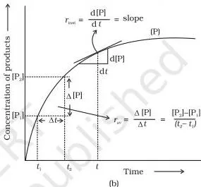
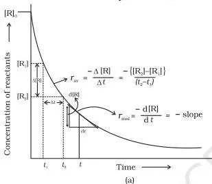
A chord drawn across the interval \(t_1 \to t_2\) has slope equal to the average rate over that window. A tangent at one point has slope equal to the instantaneous rate at exactly that instant.
The two differ because the curve is not straight: any wide interval averages fast early behaviour with slow later behaviour, so the tangent is the better answer to “what is the rate right now?”.
Fig. 3.2 applies the tangent method to real data.
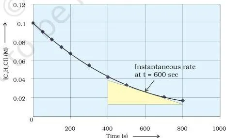
To find the instantaneous rate at 600 s, you draw a tangent at that point, read two concentration-time points the tangent passes through, and compute \(-\Delta[\text{C}_4\text{H}_9\text{Cl}]/\Delta t\). The book obtains about \(5.12 \times 10^{-5}\ \text{mol L}^{-1}\text{s}^{-1}\).
The same method at 250 s, 350 s and 450 s gives \(1.22 \times 10^{-4}\), \(1.0 \times 10^{-4}\) and \(6.4 \times 10^{-5}\ \text{mol L}^{-1}\text{s}^{-1}\) — a steady fall as reactant is used up. When a question hands you a concentration-time curve, the tangent slope is the skill being tested.
Straight-Line Plots That Identify the Order
These three graphs are the fastest way to identify an order from data. Whichever plot comes out straight tells you the order.
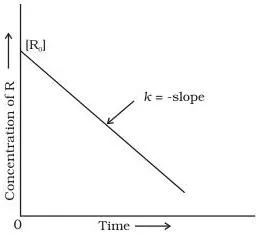
Fig. 3.3 — zero order: [R] vs t is a straight line with slope \(-k\) and intercept \([\text{R}]_0\). A linear decrease at constant rate is the signature of a reaction whose rate never changes, however much reactant remains.
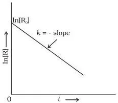
Fig. 3.4 — first order: ln[R] vs t is a straight line with slope \(-k\) and intercept \(\ln[\text{R}]_0\), matching the form \(y = mx + c\) of Eq. 3.9.
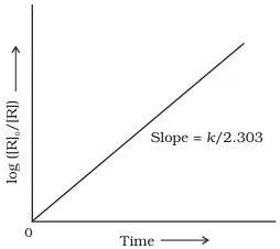
Fig. 3.5 — first order again: \(\log([\text{R}]_0/[\text{R}])\) vs t is a straight line through the origin with slope \(k/2.303\), the graph that matches Eq. 3.15 directly. Exercise 3.15 gives you N2O5 data and asks for a plot of [N2O5] against t and of log[N2O5] against t.
The second plot is the straight one; its slope yields k, and the half-life read from the concentration curve should match \(0.693/k\).
Energy Diagrams and the Maxwell-Boltzmann Curves
The next five figures sit behind the Arrhenius equation: what activation energy is, why only some molecules react, and why a 10 K rise roughly doubles the rate.
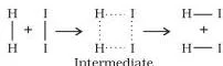
Fig. 3.6 shows the act of collision: an H2 molecule and an I2 molecule meet, form an unstable intermediate — the activated complex — and the complex breaks apart into two HI molecules. This intermediate lasts a very short time, which is why the energy to reach it matters.
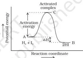
Fig. 3.7 is the reaction energy profile. The horizontal axis is reaction coordinate — progress of the reaction, not time. The curve rises from the reactants’ energy up to the activated complex: that rise is \(E_a\). It then falls to the products’ energy, and the net drop between the two valleys is the enthalpy change of the reaction.
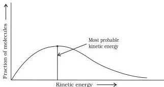
Fig. 3.8 is the Maxwell-Boltzmann energy distribution: the fraction of molecules \(N_E/N_T\) against kinetic energy. The peak is the most probable kinetic energy. The important region is to the right of \(E_a\) — the fraction of molecules carrying at least the activation energy, the only ones that can react when they collide.
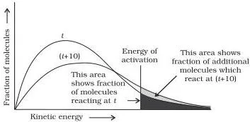
Fig. 3.9 explains the “10° doubles the rate” rule in five steps:
- At the higher temperature \(t + 10\), the maximum of the curve moves right — the most probable kinetic energy rises.
- The curve broadens and spreads to the right — a greater proportion of molecules carry high energies.
- The area under the curve stays constant, because the total probability must always be one.
- Mark \(E_a\) on the curve: the area to its right is the fraction of molecules with energy equal to or greater than \(E_a\).
- At \(t + 10\) that shaded fraction is roughly double its size at t — so the rate constant nearly doubles, exactly as the chapter states in Section 3.4.
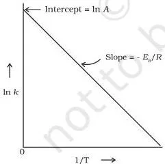
Fig. 3.10 is how \(E_a\) and A are actually measured: \(\ln k\) vs \(1/T\) is a straight line with slope \(-E_a/R\) and intercept \(\ln A\). Exercise 3.22 asks you to draw exactly this graph from N2O5 data and read both quantities off it.
Catalyst and Molecular Orientation
The last two figures close the chapter’s story: how a catalyst changes the energy picture, and why orientation decides whether a collision counts.
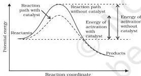
Fig. 3.11 shows two humps between the same reactants and products: the higher one is the uncatalysed path, the lower one the catalysed alternative pathway. Because \(E_a\) is smaller on the catalysed route, the Arrhenius equation gives a larger k — less energy is demanded of each colliding pair.
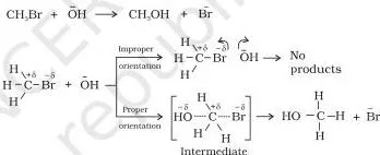
Fig. 3.12 is the reason collision theory needs the steric factor \(P\): with proper orientation, the colliding molecules form bonds and products; with improper orientation, they simply bounce back. In the rate expression \(\text{Rate} = PZ_{AB}e^{-E_a/RT}\), \(P\) corrects the collision frequency for collisions wasted on wrong orientation.
Key Terms in Chemical Kinetics, Defined
This glossary gives the precise meaning of every term the chapter uses, each tied to its section, in one line. Learn the definitions in the chapter’s own words from the PDF; use this table for quick recall.
| Term | One-line meaning |
|---|---|
| Rate of a reaction | Change in concentration of a reactant or product per unit time — a decrease for reactants, an increase for products (Section 3.1) |
| Average rate | Rate over a finite time interval, found from \(-\Delta[\text{R}]/\Delta t\) (Eq. 3.1) |
| Instantaneous rate | Rate at one instant, found as the slope of a tangent, \(-d[\text{R}]/dt\) (Eq. 3.3) |
| Rate law (rate expression) | Expression giving reaction rate in terms of reactant concentrations, each raised to an experimental power (Section 3.2.2) |
| Rate constant k | Proportionality factor in the rate law; constant for a reaction at a given temperature (Section 3.2.2) |
| Order of a reaction | Sum of the exponents in the rate law; can be 0, 1, 2, 3, fractional or negative (Section 3.2.3) |
| Molecularity | Number of reacting species that must collide simultaneously in one elementary reaction; only 1, 2, 3 (Section 3.2.4) |
| Elementary reaction | A reaction that is completed in a single step (Section 3.2.3) |
| Complex reaction | A reaction that proceeds through a sequence of elementary steps (its mechanism) (Section 3.2.3) |
| Rate determining step | The slowest step of a complex reaction, which controls the overall rate (Section 3.2.4) |
| Integrated rate equation | Integrated form of the rate law linking concentrations at different times to k (Section 3.3) |
| Half-life \(t_{1/2}\) | Time for the reactant concentration to fall to half its initial value (Section 3.3.3) |
| Pseudo first order reaction | A higher-order reaction that follows first order kinetics because one reactant is in large excess (Section 3.3.3) |
| Activation energy \(E_a\) | Minimum energy required for reaction — the energy of the activated complex minus the energy of the reactants (Section 3.4) |
| Activated complex | Short-lived, unstable intermediate formed during a collision before products appear (Section 3.4) |
| Arrhenius factor (frequency factor) A | Constant specific to a reaction; related to collision frequency (Section 3.4) |
| Collision frequency Z | Number of collisions per second per unit volume of the reaction mixture (Section 3.5) |
| Effective collision | Collision with sufficient energy and proper orientation that leads to products (Section 3.5) |
| Steric factor P | Probability factor accounting for the correct orientation of colliding molecules (Section 3.5) |
| Catalyst | Substance that increases rate without permanent chemical change; lowers \(E_a\) (Section 3.4.1) |
| Inhibitor | Substance that reduces the rate of a reaction (Section 3.4.1) |
Key Formulas: Symbols, Units and When to Use Them
This table gathers the working equations of Chapter 3 so a numerical problem can be matched to the right formula fast. Every symbol is explained; the units column is your first check that the answer looks sane.
| Formula | Meaning of symbols | Units of k | When it applies |
|---|---|---|---|
| \(\text{Rate} = -\dfrac{d[\text{R}]}{dt} = \dfrac{d[\text{P}]}{dt}\) | [R], [P]: molar concentrations of reactant and product | Rate in \(\text{mol L}^{-1}\text{s}^{-1}\) (or \(\text{atm s}^{-1}\) for gases) | Instantaneous rate of any reaction (Eq. 3.3) |
| \(\text{Rate} = k[\text{A}]^x[\text{B}]^y\) | k: rate constant; x, y: experimental exponents | Depends on order, n = x + y | Differential rate law of any reaction (Eq. 3.4) |
| \([\text{R}] = [\text{R}]_0 – kt\); \(k = \dfrac{[\text{R}]_0 – [\text{R}]}{t}\) | [R]₀: initial concentration | \(\text{mol L}^{-1}\text{s}^{-1}\) | Zero order reactions (Eqs. 3.6–3.7) |
| \(k = \dfrac{2.303}{t}\log\dfrac{[\text{R}]_0}{[\text{R}]}\); \([\text{R}] = [\text{R}]_0 e^{-kt}\) | [R]₀, [R]: concentrations at time 0 and t | \(\text{s}^{-1}\) | First order reactions (Eqs. 3.14–3.15) |
| \(t_{1/2} = \dfrac{[\text{R}]_0}{2k}\) | [R]₀: initial concentration | k as for zero order | Zero order half-life |
| \(t_{1/2} = \dfrac{0.693}{k}\) | k: first order rate constant | k as for first order | First order half-life (Eq. 3.17) |
| \(p_{\text{A}} = 2p_i – p_t\); \(k = \dfrac{2.303}{t}\log\dfrac{p_i}{p_{\text{A}}}\) | \(p_i\): initial pressure of A; \(p_t\): total pressure at time t | \(\text{s}^{-1}\) | First order gas reaction \(\text{A(g)} \to \text{B(g)} + \text{C(g)}\) (Eq. 3.16) |
| \(k = A e^{-E_a/RT}\) | A: Arrhenius/frequency factor; \(E_a\): activation energy in J mol⁻¹; R = 8.314 J K⁻¹ mol⁻¹; T in kelvin | Same as k for the order | Temperature dependence of any rate constant (Eq. 3.18) |
| \(\log\dfrac{k_2}{k_1} = \dfrac{E_a}{2.303R}\left(\dfrac{1}{T_1} – \dfrac{1}{T_2}\right)\) | \(k_1\), \(k_2\): rate constants at \(T_1\), \(T_2\) | Ea comes out in J mol⁻¹ | k known at two temperatures (Eq. 3.22) |
| \(\text{Rate} = P Z_{AB} e^{-E_a/RT}\) | P: steric factor; \(Z_{AB}\): collision frequency | As for the order | Bimolecular elementary reaction by collision theory |
General rule for units of k for any order: from \(k = \dfrac{\text{Rate}}{[\text{A}]^n}\), where n is the order of the reaction, the units are \((\text{mol L}^{-1})^{1-n}\text{s}^{-1}\). This gives \(\text{mol L}^{-1}\text{s}^{-1}\) for n = 0, \(\text{s}^{-1}\) for n = 1, and \(\text{mol}^{-1}\text{L s}^{-1}\) for n = 2 — the three entries of Table 3.3.
A rate constant’s units alone can identify the order, as Example 3.4 demonstrates.
Three substitution warnings: \(\log\) (base 10) in Eq. 3.15 needs the 2.303 factor while \(\ln\) does not; temperatures in the Arrhenius equations are in kelvin; and \(E_a\) must be in joules when R is in \(\text{J K}^{-1}\text{mol}^{-1}\).
Common Mistakes Students Make in Chemical Kinetics
Each error below is one this chapter’s own examples and points of caution warn about. Name the mistake before you make it.
| Mistake | Correct rule | How to check your answer |
|---|---|---|
| Writing the rate law from the balanced equation | Order comes from experiments only — the rate law can never be predicted from the equation (Section 3.2.2) | Ask: were the exponents measured from data? CHCl₃ + Cl₂ has exponent 1/2; KClO₃ + 6FeSO₄ looks 10th order but is 2nd |
| Confusing order with molecularity | Order can be 0, fractional or negative and applies to complex reactions; molecularity is only 1–3 and only for elementary steps (Sections 3.2.3, 3.2.4) | Ask: is the step an elementary reaction? If not, molecularity has no meaning |
| Forgetting the 2.303 when switching between ln and log₁₀ | \(k = \dfrac{2.303}{t}\log\dfrac{[\text{R}]_0}{[\text{R}]}\) uses log₁₀; \(k = \dfrac{1}{t}\ln\dfrac{[\text{R}]_0}{[\text{R}]}\) uses ln | If you used \(\log_{10}\) and did not multiply by 2.303, k is too small by the factor 2.303 |
| Writing the wrong units for k | Units follow the order: \(\text{mol L}^{-1}\text{s}^{-1}\) for zero, \(\text{s}^{-1}\) for first, \(\text{mol}^{-1}\text{L s}^{-1}\) for second (Table 3.3) | Use \(k = \dfrac{\text{Rate}}{[\text{A}]^n}\) and cancel units — never guess from memory |
| Assuming half-life always depends on initial concentration | True only for zero order (\(t_{1/2} = [\text{R}]_0/2k\)); first order \(t_{1/2} = 0.693/k\) is independent of concentration | Write the order first, then choose the half-life formula |
| Mixing kilojoules with joules in the Arrhenius equation | R is in \(\text{J K}^{-1}\text{mol}^{-1}\), so \(E_a\) must be in joules; Example 3.10 converts 209 kJ to 209 000 J | Compare the units of \(E_a\) and R before substituting — kJ in, J in R, answer wrong |
| Using the total pressure as the reactant’s pressure in gas kinetics | Derive the reactant pressure first: for A(g) → B(g) + C(g), \(p_{\text{A}} = 2p_i – p_t\) (Eq. 3.16) | In Exercise 3.21-type problems, the measured total pressure always exceeds the reactant pressure — they are never the same number |
| Misreading the sign of the ln k vs 1/T slope | Slope = \(-E_a/R\) (Eq. 3.19), so \(E_a\) comes out positive | If your \(E_a\) is negative, you dropped the minus sign of the slope |
Exam-Focused Notes: Skills the Exercises Test
Textbook contents and the examinable syllabus are not always identical — check the current official CBSE syllabus before planning revision. Within the chapter, the thirty numbered exercises (3.1–3.30) practise a small set of skills, and each skill maps to the formulas above.
| Skill the exercises test | What to use | Representative NCERT exercises |
|---|---|---|
| Order and dimensions of k from rate expressions | Order = sum of exponents; units from \((\text{mol L}^{-1})^{1-n}\text{s}^{-1}\) | 3.1, 3.2, 3.12 |
| Rate from concentration data | Average and instantaneous rate definitions (Eqs. 3.1–3.3) | 3.8, 3.9, 3.11 |
| Order from experimental data tables | Compare rates while one concentration is held fixed | 3.10, 3.11, 3.12 |
| Half-life and decay problems | \(t_{1/2} = 0.693/k\) and \(k = \dfrac{2.303}{t}\log\dfrac{[\text{R}]_0}{[\text{R}]}\) | 3.13, 3.14, 3.16, 3.17, 3.19 |
| Gas-phase pressure method | \(p_{\text{A}} = 2p_i – p_t\) and Eq. 3.16 | 3.20, 3.21 |
| Arrhenius equation, \(E_a\) and A | Eqs. 3.18, 3.19, 3.22; kJ → J conversion | 3.22, 3.23, 3.26, 3.27, 3.28, 3.29, 3.30 |
A sensible revision order: rate and its units first, then rate law and order, then integrated equations, then half-life, then the Arrhenius equation — each step supplies the notation the next one needs. The chapter itself points out that logarithms are reviewed in Appendix IV, so practise log₁₀ arithmetic before attempting the numericals.
Chemical Kinetics: The Chapter’s Key Takeaways
Ten lines for the last read the night before, distilled from the chapter’s closing Summary.
- Chemical kinetics is the study of reaction rates, the variables that affect them, and the formation of intermediates.
- Rate is change in concentration per unit time: a decrease for reactants (with a minus sign) or an increase for products.
- Rate can be an average over an interval or an instantaneous rate — the slope of a tangent at one instant.
- The rate law is experimental and can never be predicted from the balanced chemical equation.
- Order is the sum of the concentration exponents in the rate law — 0, 1, 2, 3, fractional or negative; molecularity is only 1–3 and exists only for elementary reactions, where it equals the order.
- The rate constant k is the proportionality factor in the rate law; its units depend on the order.
- Integrated rate equations connect concentrations, time and k: zero order gives \([\text{R}] = [\text{R}]_0 – kt\); first order gives \(k = \dfrac{2.303}{t}\log\dfrac{[\text{R}]_0}{[\text{R}]}\).
- Half-life: zero order \(t_{1/2} = [\text{R}]_0/2k\); first order \(t_{1/2} = 0.693/k\), independent of concentration.
- Arrhenius equation \(k = Ae^{-E_a/RT}\): \(E_a\) is the energy difference between the activated complex and the reactants, and A is the frequency factor.
- Raising temperature or lowering \(E_a\) increases the rate; a catalyst lowers \(E_a\) through an alternative pathway and changes neither \(\Delta G\) nor the equilibrium constant.
- Collision theory adds orientation through the steric factor P: \(k = PZ_{AB}e^{-E_a/RT}\).
Related NCERT Chapters and Resources
Chapter 3 sits in the middle of Class 12 chemistry. To move backwards, revisit Chapter 2, Electrochemistry — electrochemistry and kinetics both lean on concentration, temperature and rate. The Class 12 Chemistry Part I book page lists every chapter in this part, and the Class 12 Chemistry hub covers the subject as a whole.
For condensation-style revision after the chapter, the CBSE Class 12 Chemistry notes compress each chapter for fast recall. They sit inside the wider Class 12 notes and the main CBSE notes index. Later in the Class 12 course you will meet alcohols, phenols and ethers and the d- and f-block elements, which apply the same discipline of rate, mechanism and conditions.
Sources and Data Verification
- The sections, figures, tables and exercises described here come from the NCERT Chemistry Part I textbook, Class 12, Chapter 3 Chemical Kinetics, official PDF on ncert.nic.in.
- This page covers Chapter 3 only — its sections, figures, worked examples and the exercise set printed in that chapter. It does not describe Chemistry Part II or CBSE syllabus documents.
- The page is maintained for the 2026-27 NCERT reprint and the textbook files NCERT publishes for it.
- NCERT settles textbooks, editions and PDFs; CBSE settles curriculum, syllabus and examinations.
You can verify any chapter against the official NCERT textbook portal at ncert.nic.in.
Reference: NCERT Class 12 Chemistry textbook, chapter 3, official edition on ncert.nic.in.
Chemical Kinetics Class 12: Frequently Asked Questions
What is the difference between order and molecularity of a reaction?
Answer: Order is the sum of the exponents in the experimentally determined rate law; it can be 0, fractional or even negative, and it applies to both elementary and complex reactions. Molecularity is the number of reacting species that must collide simultaneously in one elementary step; it is only 1, 2 or 3, and it applies only to elementary reactions.
For an elementary reaction the two are equal; for a complex reaction, the order is fixed by the slowest (rate-determining) step.
What is the unit of the rate constant for a first order reaction?
Answer: \(\text{s}^{-1}\). From \(k = \dfrac{\text{Rate}}{[\text{A}]}\), the concentration units cancel: \(\dfrac{\text{mol L}^{-1}\text{s}^{-1}}{\text{mol L}^{-1}} = \text{s}^{-1}\) (Table 3.3). Because the units of k depend only on the order, a rate constant given as \(\text{s}^{-1}\) identifies a first order reaction — the reasoning behind Example 3.4.
Why can the rate law not be written from the balanced chemical equation?
Answer: Because the balanced equation summarises only the overall reaction, while the reaction actually runs through several elementary steps whose slowest one decides the rate. The exponents in the rate law therefore reflect the mechanism, not the stoichiometric coefficients.
The evidence in Section 3.2.2: \(\text{CHCl}_3 + \text{Cl}_2\) has an experimental exponent of 1/2 on Cl2, and \(\text{KClO}_3 + 6\text{FeSO}_4 + 3\text{H}_2\text{SO}_4\) looks tenth order from its equation but is experimentally second order. Only experiments fix the exponents.
Why is the half-life of a first order reaction independent of initial concentration?
Answer: Substituting \([\text{R}] = [\text{R}]_0/2\) at \(t = t_{1/2}\) into \(k = \dfrac{2.303}{t}\log\dfrac{[\text{R}]_0}{[\text{R}]}\) gives \(t_{1/2} = \dfrac{2.303}{k}\log 2 = \dfrac{0.693}{k}\) (Eq. 3.17). The initial concentration cancels inside the ratio, so the half-life depends only on k. Contrast the zero order case, where \(t_{1/2} = [\text{R}]_0/2k\) grows with the starting amount.
What is a pseudo first order reaction?
Answer: A reaction that is truly higher order but obeys first order kinetics because one reactant is present in such huge excess that its concentration barely changes. The chapter’s example: hydrolysing 0.01 mol of ethyl acetate in 10 mol of water — the water falls only from 10 mol to 9.99 mol, so the rate follows the ester alone (Section 3.3.3).
Inversion of cane sugar is another pseudo first order reaction.
How do you calculate activation energy from rate constants at two temperatures?
Answer: Use the two-temperature form of the Arrhenius equation (Eq. 3.22): \(\log\dfrac{k_2}{k_1} = \dfrac{E_a}{2.303R}\left(\dfrac{1}{T_1} – \dfrac{1}{T_2}\right)\). Substitute the two rate constants and temperatures, take log₁₀ of the ratio, and solve for \(E_a\) — but convert \(E_a\) to joules before substituting, because \(R = 8.314\ \text{J K}^{-1}\text{mol}^{-1}\).
Example 3.10 applies this with 209 kJ converted to 209 000 J; the worked example in the Arrhenius section above shows the full calculation with new numbers.
Reference: NCERT Class 12 Chemistry textbook, chapter 3, official edition on ncert.nic.in.
Explore Class 12 Chemistry Books
Class 12 Chemistry on LearnCBSE:
Related chapters: