
The types of solutions class 12 students meet in chemistry are the opening topic of NCERT Chemistry Part 1. Chapter 1 is the unit Solutions, and its first section, 1.1 Types of Solutions, sorts the mixtures the whole unit studies.
This page offers the official chapter PDF and then explains what the chapter contains — concentration units, Henry’s and Raoult’s laws, colligative properties and the van’t Hoff factor — so you can revise from this page or straight from the book. It describes the current NCERT edition of Class 12 Chemistry Part 1.
Download the Types of Solutions Class 12 Chapter PDF
Open the NCERT Class 12 Chemistry Chapter 1 Types of Solutions PDF from ncert.nic.in — this is the complete first chapter of Chemistry Part 1, the unit Solutions, and it is the same file that appears in the printed book.
Save it or read it in the browser; the file runs from the opening classification of solution types to the closing exercises of the unit.
| What the chapter holds | Count | Where it is used |
|---|---|---|
| Printed pages | 30 | |
| Sections in the chapter | 18 | |
| Figures with NCERT captions | 11 | |
| Tables | 5 | |
| Worked examples | 10 | solved step by step in our NCERT Solutions |
| Exercise questions | 41 | answered in our NCERT Solutions |
| Official NCERT PDF | Download the chapter PDF | the chapter exactly as NCERT publishes it |
Chapter at a Glance: What Is Inside the PDF
This table lists what the file actually holds — its sections, figures, worked examples, tables and exercise questions — so you know the size of the chapter before you open it.
What NCERT Class 12 Chemistry Chapter 1 Covers
The chapter is organised into seven teaching blocks. Knowing where each idea lives makes it easier to study the unit in order.
| Chapter block | NCERT section | What it teaches |
|---|---|---|
| Classification of solutions | 1.1 | Homogeneous mixtures; solute vs solvent; the nine solid–liquid–gas combinations; binary solutions |
| Expressing concentration | 1.2 | Mass %, volume %, mass by volume %, ppm, mole fraction, molarity, molality — and which depend on temperature |
| Solubility and Henry’s law | 1.3 | Saturation, like dissolves like, pressure and temperature effects on gases, \(p = K_H x\) |
| Vapour pressure and Raoult’s law | 1.4 | \(p_1 = p_1^0 x_1\), total pressure of volatile binary mixtures, vapour composition, non-volatile solutes |
| Ideal and non-ideal solutions | 1.5 | \(\Delta_{\text{mix}}H = 0\) and \(\Delta_{\text{mix}}V = 0\), positive and negative deviation, azeotropes |
| Colligative properties and molar mass | 1.6 | Relative lowering of vapour pressure, \(\Delta T_b\), \(\Delta T_f\), osmotic pressure |
| Abnormal molar masses and van’t Hoff factor | 1.7 | Dissociation vs association, \(i =\) normal molar mass ÷ abnormal molar mass, modified equations |
The chapter ends with its own Summary, a full exercise set and answers to selected intext questions — the exercises are the practice ground for every calculation pattern in the table above.
Key Concepts in Types of Solutions
These are the ideas the chapter is built on, in the order the book develops them. Read them in sequence, because later blocks use the vocabulary and formulas of the earlier ones.
Solutions, Solutes and Solvents
Before any calculation you need the vocabulary. A solution is a homogeneous mixture — its composition and properties are uniform throughout (NCERT Section 1.1).
The component present in the largest quantity is the solvent, and it decides the physical state of the solution. The other components are solutes.
This unit studies only binary solutions — exactly two components. Each component can be solid, liquid or gas, which gives the nine combinations of Table 1.1:
| Type of solution | Solute | Solvent | Example |
|---|---|---|---|
| Gaseous | Gas | Gas | Mixture of oxygen and nitrogen gases |
| Gaseous | Liquid | Gas | Chloroform mixed with nitrogen gas |
| Gaseous | Solid | Gas | Camphor in nitrogen gas |
| Liquid | Gas | Liquid | Oxygen dissolved in water |
| Liquid | Liquid | Liquid | Ethanol dissolved in water |
| Liquid | Solid | Liquid | Glucose dissolved in water |
| Solid | Gas | Solid | Solution of hydrogen in palladium |
| Solid | Liquid | Solid | Amalgam of mercury with sodium |
| Solid | Solid | Solid | Copper dissolved in gold |
Seven Ways to Express Concentration
Concentration answers one question: how much solute sits in a given amount of solution or solvent. The chapter gives seven units, and the exam-critical difference between them is which ones change when the temperature changes.
| Unit | What it measures | Formula | Changes with temperature? |
|---|---|---|---|
| Mass percentage (w/w) | Mass of component per 100 units of total solution mass | \(\frac{\text{mass of component}}{\text{total mass of solution}} \times 100\) | No |
| Volume percentage (v/v) | Volume of component per 100 units of total solution volume | \(\frac{\text{volume of component}}{\text{total volume of solution}} \times 100\) | Not discussed in the chapter |
| Mass by volume percentage (w/V) | Mass of solute dissolved in 100 mL of solution | — | Not discussed in the chapter |
| Parts per million (ppm) | Parts of the component per \(10^6\) parts of all components | \(\frac{\text{parts of component}}{\text{total parts}} \times 10^6\) | No |
| Mole fraction (x) | Moles of a component ÷ total moles of all components | \(x_i = \frac{n_i}{\sum n_i}\) | No; all mole fractions sum to 1 |
| Molarity (M) | Moles of solute per litre of solution | \(M = \frac{n_2}{V\ (\text{L})}\) | Yes — volume depends on temperature |
| Molality (m) | Moles of solute per kilogram of solvent | \(m = \frac{n_2}{w_1\ (\text{kg})}\) | No |
NCERT is explicit about temperature behaviour in Section 1.2: mass %, ppm, mole fraction and molality are independent of temperature, while molarity depends on temperature because volume depends on temperature and mass does not. The book does not discuss temperature effects for volume % and mass-by-volume %.
Also remember the built-in check: mole fractions in a solution always add up to 1 (equation 1.7). Use it every time you compute a mole fraction.
Worked example (original numbers). Calculate the mole fraction of ethanol (\(C_2H_5OH\), \(M = 46\ \text{g mol}^{-1}\)) in a solution made by mixing 9.2 g of ethanol with 54.0 g of water.
Step 1: Convert each mass to moles.
\[ n_{\text{ethanol}} = \frac{9.2\ \text{g}}{46\ \text{g mol}^{-1}} = 0.20\ \text{mol} \]
\[ n_{\text{water}} = \frac{54.0\ \text{g}}{18\ \text{g mol}^{-1}} = 3.0\ \text{mol} \]
Step 2: Apply the mole fraction formula.
\[ x_{\text{ethanol}} = \frac{0.20}{0.20 + 3.0} = \frac{0.20}{3.2} = 0.0625 \]
Step 3: Check with the other component.
\[ x_{\text{water}} = \frac{3.0}{3.2} = 0.9375 \quad \Rightarrow \quad x_{\text{ethanol}} + x_{\text{water}} = 1.000 \]
Final answer: \(x_{\text{ethanol}} = 0.0625\) (and \(x_{\text{water}} = 0.9375\)).
Solubility and Henry’s Law
Solubility is the maximum amount of a substance that can dissolve in a specified amount of solvent at a specified temperature (NCERT Section 1.3). This block matters because gases obey different rules from solids — pressure drives gas solubility but barely touches solids.
When a solid dissolves, dissolution and crystallisation run at the same rate at saturation. That dynamic equilibrium defines the saturated solution, which holds the maximum amount of solute.
The rule of thumb is like dissolves like: polar solutes dissolve in polar solvents and non-polar in non-polar — sodium chloride and sugar in water, but naphthalene and anthracene in benzene (Section 1.3.1).
For solids, temperature follows Le Chatelier’s principle: if dissolution is endothermic (\(\Delta_{\text{sol}}H \gt 0\)), solubility rises with temperature. Pressure has no significant effect on solids and liquids because they are nearly incompressible.
For gases the story flips. Solubility increases with pressure, and the quantitative law comes from Henry: the partial pressure of a gas is proportional to its mole fraction in solution (Section 1.3.2):
\[ p = K_H x \]
A higher \(K_H\) at a given pressure means lower solubility. Gas solubility falls as temperature rises — dissolving a gas resembles condensation and gives out heat — which is why aquatic life copes better in cold water.
The book applies Henry’s law to three real situations (Section 1.3.2): soft drinks are sealed under high pressure to keep \(CO_2\) dissolved; scuba divers risk the bends when nitrogen bubbles form in the blood as pressure drops; and climbers at high altitude suffer anoxia because the low partial pressure of oxygen leaves too little in the blood.
Worked example (original numbers). At 298 K, \(K_H\) for carbon dioxide in water is \(1.67 \times 10^8\ \text{Pa}\). Find the mole fraction of \(CO_2\) dissolved when the \(CO_2\) pressure above the drink is \(1.5 \times 10^5\ \text{Pa}\).
Step 1: Rearrange Henry’s law for the mole fraction.
\[ x = \frac{p}{K_H} \]
Step 2: Both pressures are in Pa, so no unit conversion is needed.
\[ x = \frac{1.5 \times 10^5\ \text{Pa}}{1.67 \times 10^8\ \text{Pa}} = 8.98 \times 10^{-4} \approx 9.0 \times 10^{-4} \]
Final answer: \(x_{CO_2} \approx 9.0 \times 10^{-4}\).
The same \(K_H\) value appears in Intext Question 1.7 of the book, where it is used for soda water packed under \(CO_2\) pressure.
Vapour Pressure and Raoult’s Law
Every liquid in a closed vessel exerts a vapour pressure, and the chapter uses it as a concentration probe. You must keep two cases separate — two volatile liquids, and a non-volatile solute in a liquid — because the equations look alike but describe different settings.
Case 1: two volatile liquids. Raoult’s law (Section 1.4.1) states that each component’s partial pressure is proportional to its mole fraction:
\[ p_1 = p_1^0 x_1 \quad \text{and} \quad p_2 = p_2^0 x_2 \]
The total pressure follows from Dalton’s law of partial pressures:
\[ p_{\text{total}} = p_1^0 + (p_2^0 – p_1^0)x_2 \]
Because \(p_i = y_i p_{\text{total}}\), the vapour composition follows from the partial pressures. The book’s conclusion after Example 1.5: at equilibrium the vapour phase is always richer in the more volatile component — the one with the higher pure vapour pressure.
Case 2: non-volatile solute in a liquid. Only the solvent appears in the vapour, so \(p_1 = x_1 p_1^0\) (Section 1.4.3). Solute particles occupy part of the surface (see Fig. 1.4 in the figure walkthrough below), fewer solvent molecules escape, and the vapour pressure of the solution is lower than that of the pure solvent.
One more connection worth noting: Raoult’s law and Henry’s law have the same shape, \(p = (\text{constant})x\). Raoult’s law is therefore a special case of Henry’s law in which the constant \(K_H\) equals the pure vapour pressure \(p_i^0\) (Section 1.4.2).
Worked example (original numbers, book’s data). Heptane and octane form an ideal solution. At 373 K their pure vapour pressures are 105.2 kPa and 46.8 kPa. Find the total vapour pressure and the vapour-phase mole fraction of heptane for a mixture of 45 g of heptane with 60 g of octane.
Step 1: Find the molar masses.
Heptane \(C_7H_{16} = 100\ \text{g mol}^{-1}\); octane \(C_8H_{18} = 114\ \text{g mol}^{-1}\).
\[ n_{\text{hep}} = \frac{45}{100} = 0.45\ \text{mol} \quad ; \quad n_{\text{oct}} = \frac{60}{114} = 0.526\ \text{mol} \]
Step 2: Mole fractions in the liquid.
\[ x_{\text{hep}} = \frac{0.45}{0.976} = 0.461 \quad ; \quad x_{\text{oct}} = 0.539 \]
Step 3: Apply Raoult’s law.
\[ p_{\text{total}} = (0.461)(105.2) + (0.539)(46.8) = 48.5 + 25.2 = 73.7\ \text{kPa} \]
Step 4: Vapour-phase mole fraction of heptane from \(y_i = p_i/p_{\text{total}}\).
\[ y_{\text{hep}} = \frac{48.5}{73.7} = 0.66 \]
Final answer: \(p_{\text{total}} = 73.7\ \text{kPa}\); the vapour holds 66% heptane although the liquid holds only 46% — the vapour is richer in the more volatile component.
Ideal Solutions, Deviations and Azeotropes
An ideal solution is a reference standard — one that obeys Raoult’s law at every concentration. Real mixtures deviate from it, and the chapter explains why using intermolecular forces.
Ideal solutions (Section 1.5.1) obey Raoult’s law over the whole concentration range with \(\Delta_{\text{mix}}H = 0\) and \(\Delta_{\text{mix}}V = 0\). This happens when A–A, B–B and A–B attractions are nearly equal — for example n-hexane and n-heptane, or benzene and toluene.
Positive deviation occurs when A–B interactions are weaker than A–A or B–B, so molecules escape more easily and the vapour pressure rises — ethanol and acetone behave this way, because acetone breaks some of ethanol’s hydrogen bonds.
Negative deviation occurs when A–B is stronger, lowering the vapour pressure — chloroform–acetone and phenol–aniline form hydrogen bonds between unlike molecules.
| Property | Ideal solution | Positive deviation | Negative deviation |
|---|---|---|---|
| A–B vs A–A and B–B interactions | Nearly equal | A–B weaker | A–B stronger |
| \(\Delta_{\text{mix}}H\) | Zero | Positive | Negative |
| \(\Delta_{\text{mix}}V\) | Zero | Positive | Negative |
| Vapour pressure vs Raoult’s law | Matches | Higher | Lower |
| Examples | n-Hexane–n-heptane; benzene–toluene | Ethanol–acetone; carbon disulphide–acetone | Chloroform–acetone; phenol–aniline |
Azeotropes (Section 1.5.2) are binary mixtures whose liquid and vapour have the same composition and which boil at a constant temperature — fractional distillation cannot separate them at that composition.
Large positive deviations give minimum boiling azeotropes such as ethanol–water (about 95% ethanol by volume); large negative deviations give maximum boiling azeotropes such as nitric acid–water (about 68% acid by mass, boiling at 393.5 K).
Colligative Properties and Molar Mass
Colligative properties are the payoff of the chapter: four properties that depend only on the number of solute particles, not their nature (Section 1.6). Each one gives a route to molar mass, which is why the section is titled “and Determination of Molar Mass”.
The four are relative lowering of vapour pressure, elevation of boiling point \(\Delta T_b = K_b m\), depression of freezing point \(\Delta T_f = K_f m\), and osmotic pressure \(\Pi = CRT\). For dilute solutions the relative lowering equals the solute mole fraction (Section 1.6.1):
\[ \frac{\Delta p_1}{p_1^0} = \frac{p_1^0 – p_1}{p_1^0} = x_2 \approx \frac{n_2}{n_1} \]
Molar masses follow directly:
\[ M_2 = \frac{1000 \times K_b \times w_2}{\Delta T_b \times w_1} \quad ; \quad M_2 = \frac{1000 \times K_f \times w_2}{\Delta T_f \times w_1} \quad ; \quad M_2 = \frac{w_2RT}{\Pi V} \]
Here \(w_1, w_2\) are the masses of solvent and solute in grams, \(M_2\) is the solute molar mass, \(m\) is molality, and \(V\) is the volume of solution in litres.
Worked example (original numbers). 34.2 g of sucrose (\(M = 342\ \text{g mol}^{-1}\)) is dissolved in 500 g of water. Given \(K_b = 0.52\ \text{K kg mol}^{-1}\), find the elevation of boiling point and the new boiling point of the solution (pure water boils at 373.15 K).
Step 1: Find the molality — moles of solute per kilogram of solvent.
\[ m = \frac{34.2/342}{0.500} = \frac{0.10}{0.500} = 0.20\ \text{mol kg}^{-1} \]
Step 2: Apply \(\Delta T_b = K_b m\).
\[ \Delta T_b = 0.52 \times 0.20 = 0.104\ \text{K} \]
Final answer: \(\Delta T_b \approx 0.10\ \text{K}\); the solution boils at \(373.15 + 0.104 = 373.25\ \text{K}\) — higher than pure water, as a non-volatile solute always makes it.
Worked example (original numbers). 12.5 g of glucose (\(M = 180\ \text{g mol}^{-1}\)) is dissolved in 250 g of water. Given \(K_f = 1.86\ \text{K kg mol}^{-1}\), find the depression of freezing point.
Step 1: Find the molality.
\[ m = \frac{12.5/180}{0.250} = \frac{0.0694}{0.250} = 0.278\ \text{mol kg}^{-1} \]
Step 2: Apply \(\Delta T_f = K_f m\).
\[ \Delta T_f = 1.86 \times 0.278 = 0.517 \approx 0.52\ \text{K} \]
Final answer: \(\Delta T_f \approx 0.52\ \text{K}\), so the solution freezes about half a degree lower than pure water.
Worked example (original numbers). A 2.0 g sample of a polymer is dissolved to make 500 mL of solution. The osmotic pressure at 300 K is 0.20 bar. Given \(R = 0.083\ \text{L bar mol}^{-1}\text{K}^{-1}\), find the polymer molar mass.
Step 1: Use \(M_2 = w_2RT/\Pi V\) with \(V = 0.500\ \text{L}\).
\[ M_2 = \frac{2.0 \times 0.083 \times 300}{0.20 \times 0.500} = \frac{49.8}{0.10} = 498\ \text{g mol}^{-1} \]
Final answer: \(M_2 \approx 498\ \text{g mol}^{-1}\).
Osmosis is the flow of solvent across a semipermeable membrane from lower to higher solute concentration (Section 1.6.4). The osmotic pressure is the excess pressure that just stops that flow.
The chapter’s blood-cell examples fix the vocabulary: two solutions with the same osmotic pressure are isotonic; one more concentrated than 0.9% (mass/volume) sodium chloride is hypertonic, and cells placed in it shrink as water leaves them; one less concentrated is hypotonic, and cells swell as water enters.
Normal saline — the 0.9% salt solution — is safe to inject intravenously because it matches the osmotic pressure of the fluid inside blood cells.
The osmotic pressure method is the chapter’s recommended route for proteins, polymers and other biomolecules (Section 1.6.4): pressure is measured near room temperature, where proteins are stable; the formula uses molarity rather than molality; and the measured pressure is large even for very dilute solutions, so experimental errors stay small.
If the applied pressure exceeds the osmotic pressure, the flow of solvent reverses — pure solvent leaves the solution through the membrane (Section 1.6.5). This reverse osmosis is used to desalinate sea water: pressure squeezes fresh water out through a cellulose acetate membrane that blocks salts and ions.
Abnormal Molar Masses and the van’t Hoff Factor
Ionic and associating solutes break the simple colligative equations. The van’t Hoff factor \(i\) accounts for the real number of particles and fixes every formula.
When KCl dissolves, each formula unit gives two ions, so the particle count doubles and colligative effects double: 1 mol of KCl in 1 kg of water raises the boiling point by about \(0.52 \times 2 = 1.04\ \text{K}\). Judged from that effect, the molar mass appears to be half the true value — this is an abnormal molar mass (Section 1.7).
Association works in reverse. Ethanoic acid dimerises in benzene through hydrogen bonding, so two molecules count as one particle. If all molecules dimerise, \(\Delta T_b\) and \(\Delta T_f\) are half the normal values and the measured molar mass is twice the expected value.
The factor is defined as (Section 1.7):
\[ i = \frac{\text{normal molar mass}}{\text{abnormal molar mass}} = \frac{\text{observed colligative property}}{\text{calculated colligative property}} \]
So \(i \gt 1\) for dissociation — about 2 for KCl, NaCl and MgSO₄, and about 3 for \(K_2SO_4\) at high dilution (Table 1.4) — while \(i \lt 1\) for association, about 0.5 for acetic acid in benzene. The modified equations are:
\[ \Delta T_b = iK_b m \quad ; \quad \Delta T_f = iK_f m \quad ; \quad \Pi = \frac{i n_2 RT}{V} \quad ; \quad \frac{\Delta p_1}{p_1^0} = \frac{i n_2}{n_1} \]
This is why benzoic acid in benzene shows a molar mass nearly double its normal value: two molecules join into one dimer, so the measured value is close to \(2 \times 122 = 244\ \text{g mol}^{-1}\). The book’s Example 1.12 measures 241.98 g mol⁻¹ and finds 99.2% association.
Worked example (original numbers). A 0.010 molal aqueous KCl solution shows a boiling point elevation of 0.0104 K. \(K_b\) for water is 0.52 K kg mol⁻¹. Find the van’t Hoff factor.
Step 1: Calculate the elevation that KCl would give without dissociation.
\[ \Delta T_b = 0.52 \times 0.010 = 0.0052\ \text{K} \]
Step 2: Divide the observed value by the calculated value.
\[ i = \frac{0.0104}{0.0052} = 2.0 \]
Final answer: \(i = 2.0\), consistent with KCl dissociating completely into two ions.
Formulas From the Chapter, With Symbols Explained
This is the night-before sheet: every key equation with each symbol’s meaning and unit, using the chapter’s own notation (\(w_1, w_2\) for masses, \(M_1, M_2\) for molar masses, \(m\) for molality).
| Quantity | Formula | What each symbol means (units) |
|---|---|---|
| Mole fraction | \(x_i = \frac{n_i}{\sum n_i}\) | \(n_i\) = moles of component i; sum of all \(x_i = 1\) (no unit) |
| Molarity | \(M = \frac{n_2}{V\ (\text{L})}\) | \(n_2\) = moles of solute; \(V\) = volume of solution in litres (mol L⁻¹) |
| Molality | \(m = \frac{n_2}{w_1\ (\text{kg})}\) | \(w_1\) = mass of solvent in kg (mol kg⁻¹) |
| Henry’s law | \(p = K_H x\) | \(p\) = partial pressure of gas; \(x\) = mole fraction of dissolved gas; \(K_H\) has the same pressure unit as \(p\) |
| Raoult’s law (volatile component) | \(p_1 = p_1^0 x_1\) | \(p_1^0\) = vapour pressure of the pure component at the same temperature |
| Total pressure, two volatile liquids | \(p_{\text{total}} = p_1^0 + (p_2^0 – p_1^0)x_2\) | \(x_2\) = liquid mole fraction of component 2 |
| Vapour composition | \(p_i = y_i p_{\text{total}}\) | \(y_i\) = mole fraction of component i in the vapour phase (Dalton’s law) |
| Relative lowering of vapour pressure | \(\frac{\Delta p_1}{p_1^0} = x_2 \approx \frac{n_2}{n_1}\) | \(\Delta p_1 = p_1^0 – p_1\); the approximation \(n_2/n_1\) holds for dilute solutions |
| Elevation of boiling point | \(\Delta T_b = K_b m\) | \(K_b\) = molal elevation constant (K kg mol⁻¹) |
| Depression of freezing point | \(\Delta T_f = K_f m\) | \(K_f\) = molal depression constant (K kg mol⁻¹) |
| Molar mass from \(\Delta T_b\) | \(M_2 = \frac{1000 \times K_b \times w_2}{\Delta T_b \times w_1}\) | Masses \(w_1, w_2\) in grams |
| Molar mass from \(\Delta T_f\) | \(M_2 = \frac{1000 \times K_f \times w_2}{\Delta T_f \times w_1}\) | Masses \(w_1, w_2\) in grams |
| Osmotic pressure | \(\Pi = CRT = \frac{n_2RT}{V}\) | \(C\) = molarity; \(R\) = gas constant chosen to match the units of \(\Pi\) and \(V\) |
| Molar mass from osmotic pressure | \(M_2 = \frac{w_2RT}{\Pi V}\) | \(w_2\) = mass of solute in grams |
| van’t Hoff factor | \(i = \frac{\text{normal molar mass}}{\text{abnormal molar mass}}\) | \(i \gt 1\) for dissociation; \(i \lt 1\) for association |
| Modified colligative equations | \(\Delta T_b = iK_b m\); \(\Delta T_f = iK_f m\); \(\Pi = \frac{i n_2 RT}{V}\) | Multiply by \(i\) wherever the particle count enters |
Reading the Chapter’s Key Figures
The chapter’s diagrams are not decoration — each one carries a concept you can state in words. These clusters group the figures by idea and explain how to read each one.
Reading the Gas Solubility Figures (Figs 1.1 and 1.2)
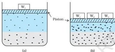
Figure 1.1 shows a gas over its solution in two states. In (a) the system sits at equilibrium; in (b) the gas has been compressed, crowding more particles above the surface so more strike the liquid each second. Equilibrium re-establishes with a higher dissolved concentration — the reason solubility rises with pressure (Section 1.3.2).
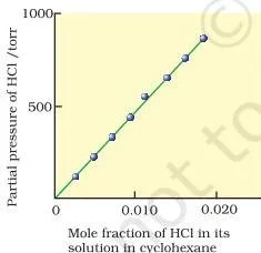
Figure 1.2 is the experimental straight line behind Henry’s law: partial pressure of HCl gas against its mole fraction in cyclohexane at 293 K. Read the slope — it is \(K_H\). A steeper slope means a bigger \(K_H\), and a bigger \(K_H\) means a smaller solubility at the same pressure.
The Ideal Solution Vapour Pressure Plot (Fig 1.3)
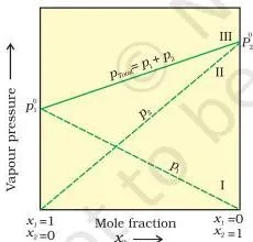
This is the master graph of Raoult’s law for two volatile liquids. Dashed line I shows \(p_1\) rising linearly with \(x_1\) from 0 to \(p_1^0\); dashed line II shows \(p_2\) falling from \(p_2^0\) to 0 as \(x_1\) grows.
Solid line III is the total pressure, running between the two pure vapour pressures — its endpoints are \(p_1^0\) and \(p_2^0\). Given the two pure pressures you can read the total pressure of any mixture off line III, or compute it from \(p_{\text{total}} = p_1^0 + (p_2^0 – p_1^0)x_2\).
Why Vapour Pressure Falls (Figs 1.4 and 1.5)
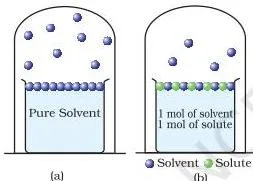
In Fig 1.4(a) the pure solvent surface is entirely solvent molecules. In (b) solute particles (dark circles) occupy part of the surface, so fewer solvent molecules escape per second and the vapour pressure drops. The drop depends on the quantity of solute particles, not their identity.
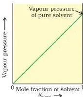
Fig 1.5 compresses that idea into one straight line: vapour pressure falls linearly from the pure solvent value \(p_1^0\) at \(x_1 = 1\) to zero at \(x_1 = 0\). The gap from the pure value is \(\Delta p_1 = x_2 p_1^0\).
Positive and Negative Deviation in One Graph (Fig 1.6)
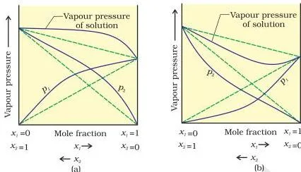
In both plots the dashed straight line is what Raoult’s law predicts. Curve (a) runs above it — the mixture gives off more vapour than ideality predicts, which is positive deviation from weaker A–B interactions. Curve (b) runs below — negative deviation from stronger A–B interactions.
When a deviation is very large, the extreme point of the curve is the azeotrope composition.
Boiling Point and Freezing Point Diagrams (Figs 1.7 and 1.8)
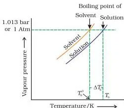
The solution’s vapour pressure curve sits below pure water’s at every temperature. Pure water boils at 373.15 K because its vapour pressure reaches 1.013 bar there; the solution reaches 1.013 bar only at a higher temperature, and the gap is \(\Delta T_b\) (Section 1.6.2).
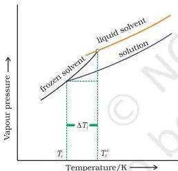
Freezing is the mirror image. A liquid freezes when its vapour pressure matches the solid’s; because the solution’s vapour pressure is lower, that equality occurs at a lower temperature, and the gap is \(\Delta T_f\). Both figures trace back to one cause — the lowered vapour pressure of the solution.
Osmosis in Three Stages (Figs 1.9, 1.10 and 1.11)
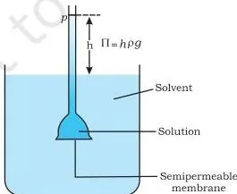
In the thistle funnel the membrane lets only solvent through, so water crosses from the beaker into the solution and the level in the stem rises. That flow is osmosis, and it always runs from lower to higher solute concentration (Section 1.6.4).
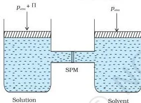
Applying pressure on the solution side slows the flow. When the applied pressure just stops it, that pressure equals the osmotic pressure \(\Pi\).
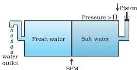
Apply a pressure larger than \(\Pi\) and the flow reverses: pure solvent leaves the solution through the membrane. This is reverse osmosis — the principle that desalination plants use to squeeze fresh water out of sea water through cellulose acetate membranes (Section 1.6.5).
Key Terms and Definitions From the Chapter
This one-line glossary fixes the vocabulary the chapter uses, in plain words, so you can answer definition questions quickly.
| Term | One-line meaning | NCERT section |
|---|---|---|
| Solution | Homogeneous mixture of two or more components | 1.1 |
| Binary solution | Solution with exactly two components | 1.1 |
| Saturated solution | Solution in dynamic equilibrium with undissolved solute, holding the maximum solute | 1.3.1 |
| Like dissolves like | Polar solutes dissolve in polar solvents, non-polar in non-polar | 1.3.1 |
| Henry’s law | At constant temperature, solubility of a gas is directly proportional to its partial pressure | 1.3.2 |
| Henry’s law constant \(K_H\) | Constant in \(p = K_H x\); larger \(K_H\) means lower gas solubility | 1.3.2 |
| Raoult’s law | Partial vapour pressure of each volatile component is proportional to its mole fraction | 1.4.1 |
| Vapour pressure | Pressure exerted by vapour in equilibrium with its liquid | 1.4.3 |
| Ideal solution | Obeys Raoult’s law at all concentrations with \(\Delta_{\text{mix}}H = 0\) and \(\Delta_{\text{mix}}V = 0\) | 1.5.1 |
| Positive deviation | Vapour pressure higher than Raoult’s law predicts; A–B weaker than A–A and B–B | 1.5.2 |
| Negative deviation | Vapour pressure lower than predicted; A–B stronger than A–A and B–B | 1.5.2 |
| Azeotrope | Binary mixture whose liquid and vapour have the same composition; boils at constant temperature | 1.5.2 |
| Colligative properties | Properties that depend on the number of solute particles, not their nature | 1.6 |
| Relative lowering of vapour pressure | \((p_1^0 – p_1)/p_1^0\), equal to the solute mole fraction | 1.6.1 |
| Elevation of boiling point | Rise in boiling point from lowered vapour pressure; \(\Delta T_b = K_b m\) | 1.6.2 |
| Depression of freezing point | Fall in freezing point from lowered vapour pressure; \(\Delta T_f = K_f m\) | 1.6.3 |
| Osmosis | Flow of solvent across a semipermeable membrane from lower to higher solute concentration | 1.6.4 |
| Semipermeable membrane | Membrane whose pores pass solvent molecules but block solute molecules | 1.6.4 |
| Osmotic pressure | Excess pressure that just stops osmosis | 1.6.4 |
| Isotonic, hypertonic, hypotonic | Same, higher or lower salt concentration than the reference fluid; 0.9% NaCl is normal saline | 1.6.4 |
| Reverse osmosis | Applying pressure greater than \(\Pi\) to push pure solvent out of a solution | 1.6.5 |
| Abnormal molar mass | Experimental molar mass lower (dissociation) or higher (association) than the true value | 1.7 |
| van’t Hoff factor \(i\) | Normal molar mass ÷ abnormal molar mass; \(i \gt 1\) for dissociation, \(i \lt 1\) for association | 1.7 |
Common Mistakes Students Make in This Chapter
Each of these errors is easy to make and easy to fix once named. Most come straight from the book’s own clarifications.
| Mistake | Correct rule | How to check your answer |
|---|---|---|
| Using volume of solution in molality and mass of solvent in molarity | Molality divides moles of solute by mass of solvent in kg; molarity divides moles by volume of solution in litres (Section 1.2) | Check the unit of the answer: molality gives mol kg⁻¹, molarity gives mol L⁻¹ |
| Assuming molarity is temperature independent | Molarity uses volume, and volume changes with temperature, so molarity changes too. Molality, mole fraction, mass % and ppm do not (end of Section 1.2) | When temperature changes, keep molality the same but recompute molarity if the volume changes |
| Mixing pressure units in Henry’s law | \(p\) and \(K_H\) must share the same pressure unit — the book converts 76.48 kbar to 76,480 bar before dividing (Example 1.4) | Convert everything (kbar, Pa, mm Hg, atm) to one unit first, then apply \(p = K_H x\) |
| Assuming the vapour phase has the same composition as the liquid | At equilibrium the vapour is always richer in the more volatile component (note after Example 1.5) | Compute \(y_i = p_i/p_{\text{total}}\); the more volatile component must have the higher \(y_i\) |
| Using the two-volatile-liquids equation for a non-volatile solute | With a non-volatile solute only the solvent contributes to vapour pressure: \(p_1 = x_1 p_1^0\) (Section 1.4.3) | Ask first: does the solute appear in the vapour? If not, it contributes no partial pressure |
| Forgetting the van’t Hoff factor for salts | 1 mol of KCl in 1 kg of water raises the boiling point by about 1.04 K, not 0.52 K, because each formula unit gives two ions (Section 1.7) | For ionic or associating solutes use \(\Delta T_b = iK_b m\) and check \(i \approx\) number of ions |
| Getting the direction of osmosis backwards | Solvent flows from lower to higher solute concentration across a semipermeable membrane (Section 1.6.4) | Test with blood cells: in hypertonic salt the cells shrink, so water must have left them |
| Using the wrong \(K_f\) or \(K_b\) for the same solvent | Values can differ between the table and an example — benzene’s \(K_f\) is 5.12 in Table 1.3 but 4.9 in Example 1.12. Use the value the question supplies | Circle the constant printed in the question and use exactly that value |
How to Revise This Chapter
This guidance is grounded in the chapter’s own structure, not in any exam prediction. Use it to plan where your practice time goes.
- Sections 1.6 and 1.7 are the calculation-heavy core. Colligative properties, molar-mass determination and the van’t Hoff factor form the longest block of worked examples in the chapter, and that is where most calculation practice belongs.
- Master the five calculation patterns: converting between concentration units; Henry’s law; Raoult’s total pressure plus vapour composition; molar mass from \(\Delta T_b\), \(\Delta T_f\) and osmotic pressure; and inserting \(i\) for electrolytes and associating solutes. Exercises 1.16 (heptane–octane), 1.19 (vapour pressure after adding water) and 1.33 (van’t Hoff factor from \(\Delta T_f\)) are representative of the three families.
- Use the book’s own self-check tools: the intext questions spread through the chapter have answers at the end of the book, and the closing exercise set gives full practice. A full-marks answer names the law or formula, substitutes with units, shows the unit cancellation, and states the final value with its unit — for colligative problems, state whether the property rises or falls.
- Textbook contents and the examinable syllabus are not always identical — check the current official CBSE syllabus before deciding what to skip.
For a second pass, pair this chapter with the CBSE Class 12 Chemistry notes hub and the wider Class 12 notes collection.
Chapter 1 Solutions: Revision Summary
This is the chapter’s own Summary (page 27 of the book) recast as a quick flow — read it the night before an assessment.
- A solution is a homogeneous mixture of two or more substances; solutions are gaseous, liquid or solid, and this chapter focuses on binary liquid solutions.
- Concentration is expressed by mole fraction, molarity, molality and the percentage units; mole fractions of all components sum to 1.
- The dissolution of a gas in a liquid follows Henry’s law: at a given temperature, the solubility of a gas is directly proportional to its partial pressure — and it falls as temperature rises.
- A non-volatile solute lowers the vapour pressure of a solvent; Raoult’s law sets the relative lowering equal to the solute’s mole fraction.
- For two volatile liquids, \(p_{\text{total}} = p_1^0 x_1 + p_2^0 x_2\), and the vapour phase is always richer in the more volatile component.
- Ideal solutions obey Raoult’s law at all concentrations; real solutions show positive or negative deviations, and very large deviations produce azeotropes.
- The four colligative properties — lowering of vapour pressure, elevation of boiling point, depression of freezing point and osmotic pressure — depend only on the number of solute particles.
- Osmosis can be reversed by a pressure greater than the osmotic pressure, which is the basis of sea-water desalination.
- Colligative properties give molar masses: dissociation lowers the observed molar mass, association raises it.
- The van’t Hoff factor \(i =\) normal molar mass ÷ abnormal molar mass = observed colligative property ÷ calculated colligative property corrects every colligative equation.
Related Class 12 Chemistry Resources
This listing is maintained for the 2026-27 academic session using the NCERT textbook information available to us. NCERT remains the authority for confirming the latest edition.
These pages take you to the rest of the book and to notes on the same material. There is no previous chapter — this is Chapter 1 of the book.
- NCERT Class 12 Chemistry Part 1 book page — every chapter of this book with its official PDF.
- Chapter 2: Electrochemistry — the next unit of Chemistry Part 1.
- Class 12 NCERT books — all subjects of this class.
- CBSE Class 12 Chemistry notes hub — chapter-wise revision notes.
- Electrochemistry CBSE notes — notes for the chapter that follows this one.
- CBSE notes library — notes across classes and subjects.
Reference: NCERT Class 12 Chemistry textbook, chapter 1, official edition on ncert.nic.in.
Sources and Data Verification
Four things you should know about this page’s basis, in plain words:
- The contents and figures on this page come from NCERT Class 12 Chemistry Part 1, Chapter 1 (Solutions), current NCERT edition, as published on the official NCERT textbook page for Class 12 Chemistry Part 1.
- This page covers this one chapter, not the rest of the book.
- This listing is maintained for the current academic session using the NCERT information available to us.
- NCERT settles textbooks, editions and PDFs; CBSE settles curriculum, syllabus and examinations.
Textbook contents and the examinable syllabus are not always identical — check the current official CBSE syllabus before deciding what to skip.
Frequently Asked Questions: Types of Solutions Class 12
Where can I download the official NCERT Class 12 Chemistry Chapter 1 Types of Solutions PDF?
Use the link at the top of this page — the official NCERT Class 12 Chemistry Chapter 1 Types of Solutions PDF is hosted on ncert.nic.in. It is the complete first chapter, the unit Solutions, from Chemistry Part 1.
Why is molarity temperature dependent but molality is not?
Because the two units are defined differently. Molarity divides moles of solute by the volume of solution in litres, and volume changes with temperature. Molality divides moles by the mass of solvent in kilograms, which does not change. NCERT states in Section 1.2 that mass %, ppm, mole fraction and molality are temperature independent, while molarity is not.
Why is the vapour phase richer in the more volatile component?
Because the more volatile component has the higher pure vapour pressure, so it contributes the larger share of the total pressure. Dalton’s law \(p_i = y_i p_{\text{total}}\) then forces its vapour-phase mole fraction \(y_i\) above its liquid mole fraction. In the book’s Example 1.5, the liquid is 68.8% CH₂Cl₂ but the vapour is 82% CH₂Cl₂.
What is the difference between an ideal and a non-ideal solution?
An ideal solution obeys Raoult’s law at all concentrations and forms with \(\Delta_{\text{mix}}H = 0\) and \(\Delta_{\text{mix}}V = 0\) — its molecules attract each other about as strongly as they attract themselves. Non-ideal solutions deviate: positive deviation raises the vapour pressure (weaker A–B attractions), negative deviation lowers it (stronger A–B attractions).
n-Hexane–n-heptane and benzene–toluene are nearly ideal; ethanol–acetone deviates positively; chloroform–acetone deviates negatively.
Why is the experimentally determined molar mass of benzoic acid in benzene nearly double its normal value?
Because benzoic acid dimerises in benzene. Benzene has a low dielectric constant, so two benzoic acid molecules join through hydrogen bonding into one dimer particle (Section 1.7). With roughly half the expected number of particles, every colligative effect is halved, and the measured molar mass comes out close to double the normal value of 122 g mol⁻¹.
The book’s Example 1.12 measures 241.98 g mol⁻¹, corresponding to 99.2% association.
What is reverse osmosis and how is it used to purify sea water?
Reverse osmosis is the reversal of osmosis: applying a pressure larger than the osmotic pressure to the solution side pushes pure solvent out of the solution through a semipermeable membrane (Section 1.6.5).
It is used to desalinate sea water — pressure squeezes fresh water through a cellulose acetate membrane that blocks salts and ions, and several countries run desalination plants this way to meet their drinking-water needs.
Explore Class 12 Chemistry Books
Class 12 Chemistry on LearnCBSE:
Related chapters: