
This is the Probability Class 12 chapter — Chapter 13 of the NCERT Class 12 Mathematics Part-II textbook — running from printed page 407 to page 438 of the book. The official NCERT PDF of the chapter is on this page, right below, so you can download it immediately. This NCERT edition carries a Reprint 2026-27 marking.
Below the download, the page explains what is inside the chapter: every section with the page it starts on, the two figures the book uses, the key definitions, and the formulas you need the night before a test.
Download the Probability Class 12 Chapter PDF (NCERT Chapter 13)
This chapter is part of Mathematics Part-II, the second NCERT Class 12 mathematics book. The official file is hosted by NCERT itself: NCERT Class 12 Mathematics Part II Chapter 13 Probability PDF.
Open it to read the chapter exactly as printed — same sections, same examples, same exercise sets — rather than a scanned or rewritten copy.
Reference: NCERT Class 12 Mathematics textbook, chapter 13, official edition on ncert.nic.in.
| What the chapter holds | Count | Where it is used |
|---|---|---|
| Printed pages | 33 | |
| Sections in the chapter | 8 | |
| Figures with NCERT captions | 2 | |
| Tables | 2 | |
| Exercise questions | 41 | answered in our NCERT Solutions |
| Official NCERT PDF | Download the chapter PDF | the chapter exactly as NCERT publishes it |
Chapter 13 Probability at a Glance
The chapter moves in a deliberate order: it builds conditional probability first, uses it to state the multiplication rule and the idea of independent events, then develops Bayes’ theorem, and closes with a summary of every formula it introduced (p. 438). The table below shows how much of each kind of content the chapter holds.
What the Probability Chapter Covers, Section by Section
This is the route the book takes — useful when you want to know where a particular idea sits before you open the PDF. Each entry names the section exactly as NCERT prints it, with the printed page it starts on.
- 13.1 Introduction (p. 407) — recaps classical and axiomatic probability and the addition rule, and promises what the chapter will do: conditional probability, then Bayes’ theorem, the multiplication rule and independence — and later the random variable, its probability distribution, and the binomial distribution.
- 13.2 Conditional Probability (pp. 407–409) — opens with the three-coin experiment (at least two heads, first coin shows tail) to show that the information “F has occurred” shrinks the sample space to F. It gives Definition 1 and, in 13.2.1, the three properties of conditional probability.
- Exercise 13.1 (pp. 413–415) — seventeen questions that drill substitution into the formula, the properties, and two multiple-choice items on when the formula is defined.
- 13.3 Multiplication Theorem on Probability (pp. 415–417) — rearranges the conditional formula into \(P(E \cap F) = P(E)P(F|E) = P(F)P(E|F)\), extends it to three events, and works two-card and three-card draws without replacement.
- 13.4 Independent Events (pp. 417–421) — the spade-ace card example shows when one event does not change another’s probability; it gives Definitions 2 and 3, the Remarks that separate independence from mutual exclusivity, and Example 13’s proof that independence of E and F carries over to E and F′ using the Venn diagram of Fig 13.3.
- Exercise 13.2 (pp. 421–423) — independence checks through the product rule, including the “odd number at least once” question whose complement form points toward binomial thinking.
- 13.5 Bayes’ Theorem (pp. 423–430) — starts from the two-bag reverse question, defines a partition of the sample space, proves the theorem of total probability, states Bayes’ theorem, runs Examples 15 through 21, and ends with the hypotheses terminology.
- Exercise 13.3 (pp. 431–433) — Bayes’ theorem in two-branch, three-branch and medical-test settings, closing with two multiple-choice items.
- Miscellaneous Examples (pp. 433–435) — Example 22’s four-box table and Example 23’s alternating throws until a six appears, which uses an infinite geometric series.
- Miscellaneous Exercise on Chapter 13 (pp. 435–437) — mixed practice from two-children phrasing to determinants and conditional-probability multiple-choice items.
- Summary (p. 438) — the chapter’s own list of every formula, in the order the chapter teaches them, followed by a short Historical Note.
Key Concepts: Conditional Probability, Independence and Bayes’ Theorem
Everything in this chapter hangs on three linked ideas: what a probability becomes when you know something has happened, when that knowledge changes nothing, and how to reverse a conditional when you observe an effect and want its cause. Each subsection below gives the formula, names every symbol, and then applies it to a worked example with fresh numbers.
Conditional probability and its three properties
The core question: once you are told that an event F has happened, the sample space is no longer S — it is F. Conditional probability measures the chance of E inside that smaller space.
Definition 1 (NCERT, p. 408): for events E and F of the same experiment, \[ P(E|F) = \frac{P(E \cap F)}{P(F)} \text{ provided } P(F) \neq 0. \]
- \(P(E \cap F)\) — the probability that both E and F occur at once;
- \(P(F)\) — the probability of the event you are conditioning on; this is the denominator;
- \(P(E|F)\) — read “probability of E given F”, the share of F’s probability that also lies in E.
Three properties follow directly from the definition (pp. 408–409):
- Property 1: \(P(S|F) = P(F|F) = 1\) — inside F, a certain event stays certain.
- Property 2: \(P((A \cup B)|F) = P(A|F) + P(B|F) – P((A \cap B)|F)\); when A and B are disjoint the last term is zero and the conditional probabilities simply add.
- Property 3: \(P(E’|F) = 1 – P(E|F)\) — because S splits into E and E′ even inside F.
Worked example (original numbers). A box holds 30 pens: 12 blue and 18 black. Four blue pens and three black pens are defective, so 7 pens are defective in all. One pen is picked at random.
Step 1: Name the events.
Let \(B\) be “the pen is black” and \(D\) be “the pen is defective”.
We want \(P(D|B)\).
Step 2: Write the known probabilities: \(P(B) = \frac{18}{30}\) and \(P(D \cap B) = \frac{3}{30}\), because 3 of the defective pens are black.
\[ P(D|B) = \frac{P(D \cap B)}{P(B)} = \frac{3/30}{18/30} = \frac{3}{18} = \frac{1}{6} \]
Check by counting: among the 18 black pens, 3 are defective, so \(P(D|B) = 3/18 = 1/6\).
The two methods agree.
Try the reverse: \(P(B|D) = \frac{P(D \cap B)}{P(D)} = \frac{3/30}{7/30} = \frac{3}{7}\).
Final answer: \(P(D|B) = \frac{1}{6}\), but \(P(B|D) = \frac{3}{7}\) — the two conditionals answer different questions, which is why the denominator must always be the probability of the conditioning event.
Independent events and the multiplication rule
Independence says the information changes nothing: knowing that F has occurred leaves E’s probability exactly where it was.
Multiplication rule (NCERT, pp. 415–416): multiply both sides of Definition 1 by \(P(F)\) to get \[ P(E \cap F) = P(E)P(F|E) = P(F)P(E|E) \text{ provided } P(E) \neq 0 \text{ and } P(F) \neq 0. \]
The rule exists because the conditional formula and the intersection formula are the same statement read two ways. For three events it extends to (p. 416):
\[ P(E \cap F \cap G) = P(E)P(F|E)P(G|EF). \]
Independence (Definitions 2 and 3, NCERT p. 418): E and F are independent when \(P(F|E) = P(F)\) and \(P(E|F) = P(E)\), which is equivalent to the product test \(P(E \cap F) = P(E)P(F)\). For three events to be mutually independent, all four conditions must hold — the three pairwise products and the triple product (p. 419).
Independence is a statement about probability, not about outcomes; that difference is the most common source of error in this chapter.
Partition, total probability and Bayes’ theorem
Bayes’ theorem answers the reverse-probability question: you observe an effect A and want to know which cause \(E_i\) produced it.
A partition of the sample space (NCERT, pp. 423–424) is a family of events \(E_1, E_2, \dots, E_n\) that are pairwise disjoint, together cover all of S, and each has nonzero probability. The simplest partition is \(\{E, E’\}\); the book also shows the four-piece family \(\{E \cap F’, E \cap F, E’ \cap F, E’ \cap F’\}\).
A partition is never unique.
Theorem of total probability (NCERT, p. 424): for any event A, \[ P(A) = \sum_{j=1}^{n} P(E_j)P(A|E_j). \]
Bayes’ theorem (NCERT, p. 425):
\[ P(E_i|A) = \frac{P(E_i)P(A|E_i)}{\sum_{j=1}^{n} P(E_j)P(A|E_j)}. \]
NCERT’s terminology (p. 426): the events \(E_i\) are called hypotheses; \(P(E_i)\) is the priori probability of the hypothesis before the experiment; \(P(E_i|A)\) is the a posteriori probability after A is known.
The book calls Bayes’ theorem the formula for the probability of ’causes’ — because exactly one \(E_i\) occurs, the formula tells you how much of the observed A was produced by each cause.
Worked example (original numbers). A factory has three machines. Machine 1 makes 50% of the output, machine 2 makes 30%, machine 3 makes 20%. Their defect rates are 2%, 3% and 4% respectively. One item is picked at random and found defective: what is the probability it came from machine 1?
Step 1: Name the partition.
\(M_1, M_2, M_3\) = “the item came from machine 1, 2, 3”, with \(P(M_1) = 0.5\), \(P(M_2) = 0.3\), \(P(M_3) = 0.2\).
These are pairwise disjoint, exhaustive and nonzero.
Step 2: Name the effect.
Let \(D\) = “the item is defective”, with \(P(D|M_1) = 0.02\), \(P(D|M_2) = 0.03\), \(P(D|M_3) = 0.04\).
Step 3: Compute the total probability — the denominator:
\[ P(D) = 0.5 \times 0.02 + 0.3 \times 0.03 + 0.2 \times 0.04 = 0.010 + 0.009 + 0.008 = 0.027. \]
Step 4: Apply Bayes’ theorem — one branch over the total:
\[ P(M_1|D) = \frac{P(M_1)P(D|M_1)}{P(D)} = \frac{0.010}{0.027} = \frac{10}{27} \approx 0.37. \]
Final answer: \(P(M_1|D) = \frac{10}{27} \approx 0.37\). Even though machine 1 makes half of all items, only about 37% of defective items come from it — because its defect rate is the lowest of the three.
Random variable
A random variable exists to turn outcomes into numbers you can do arithmetic on. NCERT’s remark (p. 431): a random variable is a real valued function whose domain is the sample space.
On the two-coin experiment with sample space \(\{HH, HT, TH, TT\}\), let X count heads: \(X(HH)=2\), \(X(HT)=1\), \(X(TH)=1\), \(X(TT)=0\). A second random variable Y can measure heads minus tails: \(Y(HH)=2\), \(Y(HT)=0\), \(Y(TH)=0\), \(Y(TT)=-2\). Two different random variables can live on the same sample space.
The chapter’s introduction (p. 407) announces what comes after it here: probability distributions of random variables and the binomial distribution.
Key Definitions in the Probability Chapter, in Plain Words
- Conditional probability (Definition 1, p. 408) — the share of F’s probability that also lies in E; defined only when \(P(F) \neq 0\).
- Independent events (Definitions 2 and 3, p. 418) — one event’s occurrence leaves the other’s probability unchanged; equivalently, \(P(E \cap F) = P(E)P(F)\).
- Partition of a sample space (pp. 423–424) — a family of nonzero events that are pairwise disjoint and together cover the whole sample space; \(\{E, E’\}\) is the basic example, and \(\{E \cap F’, E \cap F, E’ \cap F, E’ \cap F’\}\) is the book’s four-piece example.
- Priori probability (p. 426) — the probability of a hypothesis before the experiment runs.
- A posteriori probability (p. 426) — the revised probability of the hypothesis after event A is known.
- Random variable (p. 431) — a real valued function whose domain is the sample space; the two-coin X that counts heads is the book’s example.
Figure Walkthrough: Two NCERT Diagrams in This Chapter
The chapter carries several diagrams; the two below are the ones this page shows directly. The first — a Venn diagram NCERT numbers as Fig 13.3 — is not decoration: it carries the proof of Example 13. The second is the illustration NCERT places at the head of section 13.1.
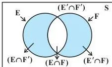
The diagram shows E divided into two pieces with no overlap: \(E \cap F\) and \(E \cap F’\), whose union is exactly E. Because the pieces are disjoint, \(P(E) = P(E \cap F) + P(E \cap F’)\). Subtract \(P(E \cap F)\) and use independence:
\[ P(E \cap F’) = P(E) – P(E)P(F) = P(E)(1 – P(F)) = P(E)P(F’). \]
That is exactly the product rule, so E and F′ are independent. The same picture returns in the common-mistakes section, because it is also the picture that separates independence from mutual exclusivity.
This is the image NCERT places at the opening of the chapter, above section 13.1. Its caption states the chapter’s starting point — probability measures the uncertainty of events in a random experiment — and the section text around it recaps the axiomatic approach of A.N. Kolmogorov that you met in earlier classes.
The image is the book’s way of saying the story continues, only now with conditions attached.
Common Mistakes Students Make in Probability Class 12
This chapter looks like simple arithmetic, but the traps are in the meaning — and NCERT’s own Remarks flag the biggest one. The list below names each mistake before you make it.
- Confusing independent with mutually exclusive. NCERT’s Remarks (pp. 418–419): independence is about probability, mutual exclusivity is about outcomes. Independent events may share outcomes — on a die, “multiple of 3” \((\{3,6\})\) and “even” \((\{2,4,6\})\) are independent and both contain 6. Two events with nonzero probabilities cannot be both independent and mutually exclusive.
- Dividing by zero. Definition 1 requires \(P(F) \neq 0\). When \(P(B) = 0\), the fraction \(P(A \cap B)/P(B)\) is not defined — Exercise 13.1 Q16 (p. 414) is built around exactly this case.
- Reversing the conditional. \(P(E|F)\) and \(P(F|E)\) answer different questions. In the chapter’s medical-test example (Example 18, pp. 426–428), the test detects 90% of HIV cases, yet the probability of actually having HIV given a positive test is about 0.083 — because the condition and the conclusion are not interchangeable.
- Letting the wording of the condition slip. “At least one boy” restricts the sample space to \(\{(b,b), (g,b), (b,g)\}\) and gives \(1/3\) (Example 2, pp. 409–410), while “elder child is a girl” leaves \(\{(g,b), (g,g)\}\) and gives \(1/2\) (Miscellaneous Q2). The condition decides the space.
- Dropping a branch of the Bayes denominator. The sum must cover every part of the partition. Example 16 (two bags, p. 426) and Example 22 (four boxes, p. 433) both fail if any \(P(E_j)P(A|E_j)\) term is left out.
| Independent events | Mutually exclusive events | |
|---|---|---|
| Meaning | Occurrence of one does not change the probability of the other (p. 418) | They share no outcome; both cannot happen together |
| Do they overlap? | Yes — they may share outcomes, such as outcome 6 in the die example | Never — \(E \cap F = \emptyset\) |
| Probability test | \(P(E \cap F) = P(E)P(F)\) | \(P(E \cap F) = 0\) with both probabilities positive |
| If both probabilities are nonzero | Then the events cannot be mutually exclusive (p. 419) | Then the events cannot be independent (p. 419) |
| Mistake | Correct rule | How to check your answer |
|---|---|---|
| Using \(P(E|F)\) when \(P(F) = 0\) | Definition 1 holds only for \(P(F) \neq 0\) (p. 408) | Confirm \(P(F) \gt 0\) before substituting; with \(P(B) = 0\) the answer is “not defined” |
| Treating \(P(E|F)\) and \(P(F|E)\) as the same | They are different fractions with different denominators | Identify which event is the condition — that event’s probability is the denominator |
| Calling mutually exclusive events independent | Independence tests \(P(E \cap F) = P(E)P(F)\); mutual exclusivity means \(E \cap F = \emptyset\) (pp. 418–419) | If the events share no outcome and both probabilities are positive, they are not independent |
| Omitting one branch of the Bayes denominator | The sum runs over every part of the partition | List all \(E_j\) first and confirm \(\sum P(E_j) = 1\) before substituting |
| Reading the condition loosely | The condition defines the restricted sample space | Write the reduced sample space and count from it, as in the two-children example |
Exam Notes for Chapter 13: How the Exercise Sets Are Built
This is a study map, not a prediction. NCERT organised the chapter’s practice into four blocks, each training a different skill; knowing which block does what lets you target your weak spot.
- Exercise 13.1 (pp. 413–415) trains the raw mechanism of conditional probability — substituting into \(P(E|F)\), applying its properties, and the multiple-choice items on the \(P(F) \neq 0\) condition.
- Exercise 13.2 (pp. 421–423) trains independence — checking \(P(E \cap F) = P(E)P(F)\) in real situations, with Q12 (p. 423), the “odd number at least once” complement question that looks forward to binomial thinking.
- Exercise 13.3 (pp. 431–433) is Bayes’ theorem in context — two-branch problems, three-branch problems, and medical-test word problems where the partition is written for you.
- Miscellaneous Exercise on Chapter 13 (pp. 435–437) mixes everything: two-children phrasing, the determinant question (Q8), the electronic-assembly question (Q9), and conditional-probability multiple-choice items (Q11–13).
A complete answer in this chapter names the events, states the formula, shows the substitution, and states the final probability as a number between 0 and 1 with one line of reasoning. The chapter’s introduction (p. 407) also says the story continues beyond this chapter: random variables, their probability distributions, and the binomial distribution come later in the book.
One honest note: textbook contents and the examinable syllabus are not always identical — check the current official syllabus before deciding what to revise.
Revision Summary: Formulas from the Chapter’s Own Summary
This checklist is rebuilt from the Summary NCERT prints on p. 438 — the book’s own list of what matters. Read each line, cover the page, and reproduce it.
- Conditional probability: \(P(E|F) = \frac{P(E \cap F)}{P(F)}\), with \(P(F) \neq 0\) mandatory.
- Bounding and algebra: \(0 \leq P(E|F) \leq 1\); complement form \(P(E’|F) = 1 – P(E|F)\); conditional addition rule \(P((E \cup F)|G) = P(E|G) + P(F|G) – P((E \cap F)|G)\).
- Multiplication rule, both orders: \(P(E \cap F) = P(E)P(F|E) = P(F)P(E|F)\), with the nonzero conditions.
- Independence: \(P(E \cap F) = P(E)P(F)\), equivalently \(P(E|F) = P(E)\) and \(P(F|E) = P(F)\).
- Theorem of total probability: \(P(A) = \sum_{j=1}^{n} P(E_j)P(A|E_j)\) over a partition.
- Bayes’ theorem: \(P(E_i|A) = \frac{P(E_i)P(A|E_i)}{\sum_{j=1}^{n} P(E_j)P(A|E_j)}\).
Use them in this order: compute the total probability first — it is the denominator — then Bayes’ theorem for the reverse question, whose numerator is a single branch of that same sum.
Related Resources and Where the Official PDF Lives
For the surrounding chapters and organised notes, use the Class 12 Mathematics notes page or the Class 12 NCERT books hub. The main CBSE notes page covers every class, and the Linear Programming notes cover the chapter that sits alongside Probability in the same book.
Sources and data verification
This page describes the NCERT Class 12 Mathematics Part-II textbook, Chapter 13 (Probability), official edition hosted by NCERT at ncert.nic.in. It covers this chapter only; the other chapters of the book are listed on the book’s index page above.
NCERT settles the textbook, its editions and the official PDFs; CBSE settles the curriculum, the syllabus and the examinations. The page references here follow the book’s own printed pagination (407–438).
Reference: NCERT Class 12 Mathematics textbook, chapter 13, official edition on ncert.nic.in.
Frequently Asked Questions on Probability Class 12
What is the difference between independent events and mutually exclusive events?
Independence is about probability; mutual exclusivity is about outcomes. Events are independent when \(P(E \cap F) = P(E)P(F)\), so knowing one happened does not change the other’s chance. Events are mutually exclusive when \(E \cap F = \emptyset\), so both cannot happen at once.
With both probabilities positive the two cannot hold together: mutual exclusivity gives \(P(E \cap F) = 0\) while \(P(E)P(F) \gt 0\).
Why is P(A|B) not defined when P(B) is zero?
Because the definition divides by \(P(B)\): \(P(A|B) = P(A \cap B)/P(B)\). A zero denominator makes the fraction meaningless, so Definition 1 (p. 408) requires \(P(F) \neq 0\). Exercise 13.1 Q16 (p. 414) tests exactly this — with \(P(A) = 1/2\) and \(P(B) = 0\), the correct option is “not defined”.
Why is the answer in the HIV test example so low even though the test is 90 percent accurate?
Because the disease is rare. With \(P(E) = 0.001\), the true-positive branch contributes \(0.001 \times 0.9 = 0.0009\), while the false-positive branch contributes \(0.999 \times 0.01 \approx 0.00999\) — more than eleven times heavier. The posterior is \(0.0009/(0.0009 + 0.00999) \approx 0.083\). Since 99.9% of people are healthy, most positive results are false positives even with an accurate test.
In a family with two children, why is the probability of both being boys 1/3 when we know at least one is a boy?
Because the condition shrinks the sample space. The full space is \(\{(b,b), (g,b), (b,g), (g,g)\}\); “at least one boy” leaves \(\{(b,b), (g,b), (b,g)\}\), of which only \(\{(b,b)\}\) is favourable, so the answer is \(1/3\) (Example 2, pp. 409–410).
If the condition were “the elder child is a girl”, the space would be \(\{(g,b), (g,g)\}\) and the answer \(1/2\). The wording of the condition decides which space you count in.
What is the difference between the theorem of total probability and Bayes theorem?
The theorem of total probability gives the overall chance of A by adding its chance over every cause: \(P(A) = \sum P(E_j)P(A|E_j)\). Bayes’ theorem answers the reverse question — given that A happened, the chance it came from a particular cause — which is that cause’s branch divided by the same total.
Ask which direction you are facing: “what is the overall chance of A?” means total probability; “given A, which cause produced it?” means Bayes’ theorem.
Explore Class 12 Mathematics Books
Class 12 Mathematics on LearnCBSE:
Related chapters: