
Application of Derivatives Class 12 is Chapter 6 of the NCERT Mathematics Part I textbook. The full official chapter runs about 40 pages and turns the differentiation rules of Chapter 5 into four practical tools: rates of change, increasing and decreasing functions, local maxima and minima, and absolute extrema on a closed interval.
The official NCERT PDF for the 2026-27 edition is linked right below, and every section, definition and key result of the chapter is explained further down this page.
Application of Derivatives Class 12: Download the Official NCERT PDF
The complete chapter, exactly as printed in the book, is a single official PDF on the NCERT website.
For a clean, print-ready copy of the text you will be examined on, download the Class 12 Mathematics Chapter 6 Application of Derivatives PDF — it carries every definition, theorem, worked example and exercise in the chapter.
The explanations on this page follow that PDF as their sole source.
| What the chapter holds | Count | Where it is used |
|---|---|---|
| Printed pages | 40 | |
| Sections in the chapter | 5 | |
| Figures with NCERT captions | 15 | |
| Tables | 5 | |
| Exercise questions | 57 | answered in our NCERT Solutions |
| Official NCERT PDF | Download the chapter PDF | the chapter exactly as NCERT publishes it |
Chapter 6 at a glance: what is inside
Chapter 6 is organised so that each new tool builds on the one before. Section 6.1 is a short introduction, Section 6.2 defines rates of change, Section 6.3 uses the sign of the derivative to find intervals where a function is increasing or decreasing, and Section 6.4 handles local and absolute maxima and minima, ending with the closed-interval working rule in Section 6.4.1.
Three numbered exercises match these sections: Exercise 6.1 on rates of change, Exercise 6.2 on increasing and decreasing functions, and Exercise 6.3 on maxima and minima. A Miscellaneous Exercise on Chapter 6 then mixes all the tools, and the chapter closes with a Summary that collects the results you are expected to keep.
The table below lists how much of the chapter there is — its sections, figures, worked examples and exercise questions.
What Application of Derivatives Class 12 covers, section by section
This chapter takes the differentiation rules you learned in Chapter 5 and uses them to answer four kinds of questions: how fast a quantity changes, where a graph rises or falls, where a function reaches its local highest and lowest points, and what its greatest and least values are on a fixed interval.
Use the section map below to jump straight to whichever part you are stuck on.
6.1 and 6.2: rates of change and related rates
If one quantity \( y \) varies with another quantity \( x \) through a rule \( y = f(x) \), then \( \frac{dy}{dx} = f'(x) \) is the rate of change of \( y \) with respect to \( x \), and \( f'(x_0) \) is that rate at \( x = x_0 \).
A positive rate means \( y \) increases when \( x \) increases; a negative rate means \( y \) decreases as \( x \) increases — a note the book states right after its first rate examples.
When both \( x \) and \( y \) are functions of time \( t \), the chain rule gives \( \frac{dy}{dx} = \frac{dy}{dt} \div \frac{dx}{dt} \), provided \( \frac{dx}{dt} \neq 0 \). The condition matters because the formula divides by \( \frac{dx}{dt} \): a zero time-rate would make the ratio meaningless.
Two economics applications appear in this section. Marginal cost is the instantaneous rate of change of total cost with respect to output, \( MC = \frac{dC}{dx} \), and marginal revenue is \( MR = \frac{dR}{dx} \), the instantaneous rate of change of total revenue with respect to units sold.
The section’s worked examples are the pattern every Exercise 6.1 question follows: a circle whose area changes with its radius, a cube of given volume growth, circular waves spreading on a lake, a rectangle whose length shrinks while its width grows, and marginal cost and revenue calculations.
Watch the sign in the rectangle problem: a length that is decreasing is a negative rate, \( \frac{dx}{dt} = -3\ \text{cm/min} \).
6.3: increasing and decreasing functions
A function is increasing on an interval when \( x_1 \lt x_2 \) gives \( f(x_1) \leq f(x_2) \), decreasing when it gives \( f(x_1) \geq f(x_2) \), and constant when \( f(x) = c \) for all \( x \). Strict inequalities define strictly increasing and strictly decreasing functions (Definition 1).
Definition 2 extends the idea to a single point: \( f \) is increasing at \( x_0 \) if it is increasing in some open interval containing \( x_0 \), and similarly for decreasing.
Theorem 1 is the working test. If \( f \) is continuous on \( [a,b] \) and differentiable on \( (a,b) \), then \( f'(x) \geq 0 \) means \( f \) is increasing on \( [a,b] \), \( f'(x) \leq 0 \) means decreasing, and \( f'(x) = 0 \) means constant.
Why the sign of \( f’ \) decides everything: the proof uses the Mean Value Theorem from Chapter 5, which gives \( f(x_2) – f(x_1) = f'(c)(x_2 – x_1) \) for some \( c \) between \( x_1 \) and \( x_2 \). The sign of \( f’ \) then fixes the sign of the change.
The book adds a generalised version: \( f'(x) \gt 0 \) on an interval, excluding the endpoints, with \( f \) continuous on the interval, is enough to conclude that \( f \) is increasing there. The \( f'(x) \lt 0 \) case is similar.
The method used in the examples — a quadratic, a cubic, \( \sin 3x \), and \( \sin x + \cos x \) — is always the same: solve \( f'(x) = 0 \), split the domain at those points, and test the sign of \( f’ \) in each interval. Listing the signs in a small table, as the book does, is the cleanest way to present the answer.
6.4: maxima and minima, local and global
The section opens with three word problems — the profit of an orange grove, the height of a thrown ball, and the distance of a helicopter from a soldier — and all three reduce to the same question: where does a function reach its largest or smallest value?
Definition 3 makes this formal: \( f \) has a maximum value \( f(c) \) on an interval \( I \) if \( f(c) \gt f(x) \) for every other \( x \) in \( I \), a minimum value if the inequality is reversed, and either one is called an extreme value.
Definition 4 introduces local maxima and minima. The point \( c \) is a point of local maxima if \( f(c) \geq f(x) \) for all \( x \) in some neighbourhood \( (c – h, c + h) \); local minima uses the reversed inequality. The comparison is only with immediate neighbours, which is what ‘local’ means.
Theorem 2 gives the key fact: if \( f \) has a local maximum or minimum at \( c \), then either \( f'(c) = 0 \) or \( f \) is not differentiable at \( c \). The converse is false — the curve \( y = x^3 \) has \( f'(0) = 0 \), yet 0 is neither a maximum nor a minimum.
Points where either condition holds are called critical points, and they are the only candidates for local extrema.
Two tests classify critical points. The First Derivative Test (Theorem 3) watches the sign of \( f’ \) as \( x \) passes through \( c \): a change from + to − gives a local maximum, − to + gives a local minimum, and no change gives a point of inflection.
The Second Derivative Test (Theorem 4) is quicker when it works: \( f'(c) = 0 \) with \( f”(c) \lt 0 \) gives a local maximum, \( f”(c) \gt 0 \) gives a local minimum, and \( f”(c) = 0 \) means the test fails — you go back to the First Derivative Test, exactly as Example 21 does.
Why the second derivative works: it measures concavity. \( f”(c) \lt 0 \) means the graph is cupped downward at \( c \), a crest; \( f”(c) \gt 0 \) means cupped upward, a trough.
The applied optimisation examples turn geometry or number puzzles into functions of one variable: two numbers whose sum of squares is minimum, the shortest distance from a point to a parabola, the trapezium of maximum area, the cylinder of greatest curved surface in a cone.
The open-box example (Example 36) adds a warning: a root can be mathematically valid but physically impossible. The root \( x = 3 \) is rejected because the aluminium sheet is only 3 m wide, so cutting 3 m squares is impossible.
6.4.1: absolute maximum and minimum on a closed interval
The book contrasts \( f(x) = x + 2 \) on the open interval \( (0,1) \), which has neither a maximum nor a minimum, with the same function on \( [0,1] \), where the greatest value is 3 at \( x = 1 \) and the least is 2 at \( x = 0 \).
On a closed interval the endpoints save you. Theorem 5 guarantees that a continuous function on \( [a,b] \) attains an absolute maximum and an absolute minimum, and Theorem 6 says that if either is attained at an interior point, the derivative is zero there.
Those two theorems produce the four-step working rule, set out in full in the core tools section below.
Miscellaneous examples and the chapter Summary
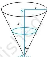
The Miscellaneous Examples combine several tools in one problem: a car whose distance–time rule gives zero velocity at both ends of its journey, an inverted cone tank filling at a fixed rate, a man walking away from a lamp post, a quartic split into four sign intervals, a heated disc expanding, the open box, and a profit maximisation problem.
Working through this set is the best rehearsal for mixed questions, because each problem makes you choose the tool rather than handing it to you.
The chapter ends with a Summary that collects every definition, theorem and the working rule. The key results section lower on this page restates that list in plainer words.
Core tools: rate of change, monotonicity and extremum tests
Most questions in Chapter 6 are one of four jobs: find a rate, decide where a function rises or falls, find a local extremum, or find an absolute extremum. Each job has one fixed tool, and the conditions attached to a tool matter as much as the formula itself.
The table below collects the tools. The worked examples after it apply each tool with fresh numbers.
| Tool | Formula or condition | What it tells you |
|---|---|---|
| Rate of change | \( \frac{dy}{dx} = f'(x) \); value at \( x_0 \) is \( f'(x_0) \) | How fast \( y \) changes per unit change in \( x \); positive means \( y \) grows with \( x \), negative means \( y \) shrinks |
| Related rates | \( \frac{dy}{dx} = \frac{dy}{dt} \div \frac{dx}{dt} \), \( \frac{dx}{dt} \neq 0 \) | Rate of \( y \) with respect to \( x \) from the two time-rates via the chain rule |
| Increasing | \( f'(x) \geq 0 \) on \( (a,b) \); strictly when \( f'(x) \gt 0 \) | The graph climbs as \( x \) increases |
| Decreasing | \( f'(x) \leq 0 \) on \( (a,b) \); strictly when \( f'(x) \lt 0 \) | The graph falls as \( x \) increases |
| Constant | \( f'(x) = 0 \) | \( f \) takes one value: \( f(x) = c \) |
| Marginal cost | \( MC = \frac{dC}{dx} \) | Extra cost of producing one more unit at output \( x \) |
| Marginal revenue | \( MR = \frac{dR}{dx} \) | Extra revenue from selling one more unit |
| First Derivative Test | \( f'(c) = 0 \); sign change + to − gives local maximum, − to + local minimum, no change inflection | Classifies a critical point by the sign behaviour of \( f’ \) |
| Second Derivative Test | \( f'(c) = 0 \) with \( f”(c) \lt 0 \) maximum, \( f”(c) \gt 0 \) minimum, \( f”(c) = 0 \) test fails | Classifies a critical point by concavity — faster when it works |
| Absolute extrema on \( [a,b] \) | Working rule: critical points, endpoints, evaluate, compare | Greatest and least values of \( f \) over the whole closed interval |
The sign of the derivative is the direction of the graph — the one memory aid the whole chapter hangs on. A positive \( f’ \) means the curve climbs, a negative \( f’ \) means it falls, and \( f’ = 0 \) means it flattens. Every test from Section 6.3 onward is that fact applied.
The closed-interval working rule
- Step 1: Find all critical points of \( f \) inside the interval — points where \( f'(x) = 0 \) or \( f \) is not differentiable.
- Step 2: Take the end points of the interval.
- Step 3: Calculate the value of \( f \) at every candidate from Steps 1 and 2.
- Step 4: Identify the largest and smallest of these values — the absolute maximum and absolute minimum of \( f \) on \( [a,b] \).
The same four steps apply whether the function is a polynomial, a trigonometric expression or a root; the only difference is how hard Step 1 is.
Worked examples: the four tools in action
Each example below uses numbers different from the book’s, so you see the method rather than a memorised answer. The working style — state the relation, differentiate, substitute, conclude — is the style exam answers should follow.
Worked example 1: rate of change of a circular ripple
A circular ripple spreads across a pond. Its radius grows at \( 2\ \text{cm/s} \). How fast is the enclosed area increasing when the radius is 6 cm?
Step 1: Write the relation.
For a circle, \( A = \pi r^2 \).
Step 2: Both \( A \) and \( r \) depend on time \( t \), so differentiate with respect to \( t \) using the chain rule:
\[ \frac{dA}{dt} = \frac{dA}{dr} \cdot \frac{dr}{dt} = 2\pi r \cdot \frac{dr}{dt} \]
Step 3: Substitute the given instant: \( r = 6\ \text{cm} \) and \( \frac{dr}{dt} = 2\ \text{cm/s} \).
\[ \frac{dA}{dt} = 2\pi(6)(2) = 24\pi \ \text{cm}^2/\text{s} \]
Final answer: the area is increasing at \( 24\pi \approx 75.4\ \text{cm}^2/\text{s} \). Substitute only after differentiating — never before.
Worked example 2: increasing and decreasing intervals
Find the intervals in which \( f(x) = x^3 – 3x^2 – 9x + 5 \) is increasing and decreasing.
Step 1: Differentiate and factor:
\[ f'(x) = 3x^2 – 6x – 9 = 3(x – 3)(x + 1) \]
Step 2: \( f'(x) = 0 \) gives the critical points \( x = -1 \) and \( x = 3 \).
These split the real line into three intervals.
Step 3: Test the sign of \( f’ \) at one point in each interval:
\[ (-\infty, -1):\ f'(-2) = 3(-5)(-1) = 15 \gt 0 \]
\[ (-1, 3):\ f'(0) = 3(-3)(1) = -9 \lt 0 \]
\[ (3, \infty):\ f'(4) = 3(1)(5) = 15 \gt 0 \]
Step 4: Read off the answer from the signs.
Final answer: \( f \) is increasing on \( (-\infty, -1) \) and \( (3, \infty) \), and decreasing on \( (-1, 3) \). The sign changes + to − at \( x = -1 \) (local maximum, value 10) and − to + at \( x = 3 \) (local minimum, value −22).
Worked example 3: second derivative test
Use the second derivative test to classify the critical points of \( f(x) = 2x^3 – 3x^2 – 12x + 7 \).
Step 1: Find the critical points.
\[ f'(x) = 6x^2 – 6x – 12 = 6(x – 2)(x + 1) \]
Step 2: So \( f'(x) = 0 \) at \( x = -1 \) and \( x = 2 \).
Now differentiate again:
\[ f”(x) = 12x – 6 \]
Step 3: Test each critical point in \( f” \):
\[ f”(-1) = -18 \lt 0 \Rightarrow \text{local maximum, value } f(-1) = 14 \]
\[ f”(2) = 18 \gt 0 \Rightarrow \text{local minimum, value } f(2) = -13 \]
Final answer: local maximum value 14 at \( x = -1 \) and local minimum value −13 at \( x = 2 \). Report the point and the value separately, as the book’s answers do.
Worked example 4: absolute extrema on a closed interval
Find the absolute maximum and minimum of \( f(x) = x^3 – 3x + 2 \) on \( [-2, 2] \).
Step 1 (critical points): \( f'(x) = 3x^2 – 3 = 3(x – 1)(x + 1) \), so the critical points are \( x = -1 \) and \( x = 1 \), both inside the interval.
Steps 2–3 (endpoints, then evaluate):
\[ f(-2) = 0, \quad f(-1) = 4, \quad f(1) = 0, \quad f(2) = 4 \]
Step 4 (compare): the largest value is 4 and the smallest is 0.
Final answer: absolute maximum value 4, attained at \( x = -1 \) and \( x = 2 \); absolute minimum value 0, attained at \( x = -2 \) and \( x = 1 \).
Notice that the maximum occurs at a critical point and at an endpoint at the same time. That is exactly why the working rule evaluates both — an absolute extremum on a closed interval has no reason to sit at a turning point.
Choosing the right test: a comparison
All three tools classify extrema, but they answer different questions, and one of them has a built-in failure mode. The table below lines them up.
| Tool | What it needs | Verdict it gives | When it fails or is unsafe |
|---|---|---|---|
| First Derivative Test | \( f \) continuous at the critical point \( c \) | Local maximum (+ to −), local minimum (− to +), inflection (no change) | Never fails for a continuous \( f \); needs sign information on both sides of \( c \) |
| Second Derivative Test | \( f \) twice differentiable at \( c \) with \( f'(c) = 0 \) | Local maximum if \( f”(c) \lt 0 \), local minimum if \( f”(c) \gt 0 \) | Fails when \( f”(c) = 0 \) — return to the first derivative test (Example 21) |
| Closed-interval working rule | \( f \) continuous on \( [a,b] \) | Absolute maximum and minimum values | No guarantee on open intervals — \( f(x) = x \) on \( (0,1) \) has neither |
Reading the graphs of Chapter 6: a figure walkthrough

![Therefore, $f'(x) = 0$ gives $\cos 3x = 0$ which in turn gives $3x = \frac{\pi}{2}, \frac{3\pi}{2}$ (as $x \in \left[0, \frac{\pi}{2}\right]$ implies $3x \in \left[0, \frac{3\pi}{2}\right]$).](https://www.learncbse.net/images/application-of-derivatives-therefore-f-x-0-gives-cos-3x-0-which-in-turn-gives-3x-frac-p.webp "Application of Derivatives Class 12: NCERT Chapter 6")
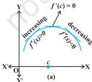
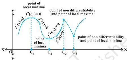
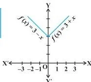
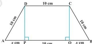

The definitions in this chapter are geometric before they are algebraic. Read the graphs first and the derivative tests stop being rules to memorise — they become facts about slopes and turning points. These are the book’s own diagrams, in the order the book uses them.
Fig 6.2: increasing, decreasing and neither, in one picture
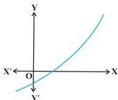
The three curves in Fig 6.2 are Definition 1 in picture form. The first graph keeps climbing from left to right — its slope is always positive, which is what \( f'(x) \gt 0 \) says. The second keeps falling, so its slope is always negative.
The third rises then falls, so it is neither: \( x_1 \lt x_2 \) does not always force \( f(x_1) \lt f(x_2) \).
Fig 6.8: the parabola of x squared — minimum value, no maximum
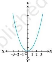
Example 14 uses Fig 6.8 to show Definition 3 in action. On the whole real line the parabola never drops below 0, so 0 is the minimum value and \( x = 0 \) is the point of minimum value. There is no maximum, because the two arms rise without bound.
The note printed under the figure is a classic exam trap: restrict the domain to \( [-2, 1] \) and the function gains a maximum value of 4, attained at the endpoint \( x = -2 \) — not at any turning point. Domains change answers, and that is the theme of Section 6.4.1.
Fig 6.9: the V-shape of the absolute value of x — an extremum without a derivative
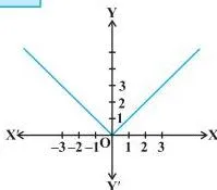
Fig 6.9 explains why a critical point is defined so broadly. The V-shape has its lowest point at \( x = 0 \), so \( |x| \) has a minimum there — but the sharp corner means \( f'(0) \) does not exist.
An extremum can sit where the derivative is zero or where it fails to exist, so the definition of a critical point bundles both cases together.
Fig 6.11: turning points — hills and valleys become local maxima and minima
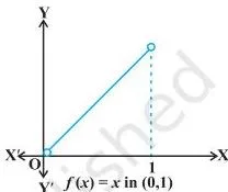
Fig 6.11 is Definition 4 without words. At A and C the graph reaches a little valley — lower than its immediate neighbours on both sides — which is exactly the inequality \( f(c) \leq f(x) \) inside \( (c – h, c + h) \). At B and D it reaches little hills.
The points are called local because the comparison covers only a small neighbourhood. A valley here can be lower than a hill far away; ‘local’ never compares across the whole domain.
The First Derivative Test reads straight off this shape: approaching A the curve falls (slope negative), leaving A it rises (slope positive), so the sign of \( f’ \) changes − to + — a local minimum.
Fig 6.13: y = x cubed — why a zero derivative is not enough
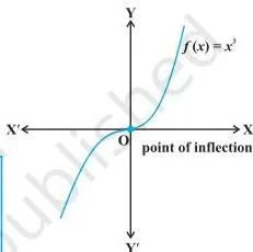
Fig 6.13 is the counterexample that stops you from reading ‘derivative zero’ as ‘turning point’. The tangent at the origin is horizontal, so \( f'(0) = 0 \), but the curve only flattens for a moment and keeps climbing.
Because \( f’ \) is positive on both sides of 0, the derivative does not change sign — no hill, no valley, just a point of inflection. This is why the First Derivative Test demands a sign change, and why the converse of Theorem 2 is false.
Fig 6.16: the two poles — a word problem becomes a function
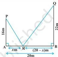
Fig 6.16 shows how a word problem becomes a function. Example 24 places poles of height 16 m and 22 m at A and B, 20 m apart, and takes a point R on AB at distance \( x \) from A.
Pythagoras then gives \( RP^2 = x^2 + 16^2 \) and \( RQ^2 = (20 – x)^2 + 22^2 \), so \( S(x) = RP^2 + RQ^2 = 2x^2 – 40x + 1140 \), a quadratic with a single minimum. The diagram is the whole trick: every applied problem in Section 6.4 is ‘express the quantity as a function of one variable, then apply the tests’.
Fig 6.23: the open box — geometry, a volume function, and a rejected root
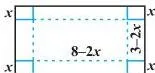
Fig 6.23 carries the geometry of Example 36. Cutting squares of side \( x \) from each corner of the 3 m by 8 m sheet leaves a box of height \( x \), breadth \( 3 – 2x \) and length \( 8 – 2x \), so its volume is \( V(x) = x(3 – 2x)(8 – 2x) \).
Setting \( V'(x) = 0 \) gives \( x = 3 \) and \( x = \frac{2}{3} \). The book asks ‘Why?’ reject \( x = 3 \): two squares of side 3 m from a sheet only 3 m wide would consume the entire width, leaving a negative breadth — physically impossible.
Only \( x = \frac{2}{3} \) survives, and the second derivative test confirms it gives the largest volume.
Key definitions you must know from Chapter 6
These are the terms the chapter defines formally, and exam answers should use them in the same sense. The most abused one is ‘critical point’ — it means a point where the derivative is zero OR does not exist, not just the first case.
| Term | What it means |
|---|---|
| Rate of change of \( y \) with respect to \( x \) | \( \frac{dy}{dx} = f'(x) \): the change in \( y \) per unit change in \( x \); \( f'(x_0) \) is the rate at \( x = x_0 \). A positive rate means \( y \) grows with \( x \); a negative rate means \( y \) shrinks. |
| Increasing / decreasing / constant on an interval | Definition 1: for \( x_1 \lt x_2 \), increasing means \( f(x_1) \leq f(x_2) \), decreasing means \( f(x_1) \geq f(x_2) \), constant means \( f(x) = c \). |
| Strictly increasing / strictly decreasing | The same with strict inequalities: \( f(x_1) \lt f(x_2) \), or \( f(x_1) \gt f(x_2) \). |
| Increasing / decreasing at a point | Definition 2: the function is increasing or decreasing in some open interval containing the point. |
| Maximum / minimum / extreme value on an interval | Definition 3: \( f(c) \gt f(x) \) for all \( x \) (maximum), \( f(c) \lt f(x) \) (minimum); either one is an extreme value. |
| Local maxima / local minima | Definition 4: \( f(c) \geq f(x) \) for all \( x \) in \( (c – h, c + h) \) (local maxima), or \( f(c) \leq f(x) \) (local minima) — comparison with immediate neighbours only. |
| Critical point | A point \( c \) where \( f'(c) = 0 \) or \( f \) is not differentiable at \( c \). |
| Point of inflection | A critical point where \( f’ \) does not change sign — the graph flattens but keeps moving in the same direction. |
| Absolute maximum / minimum on \( [a,b] \) | The greatest / least value of \( f \) over the whole closed interval; it may be attained at an endpoint. |
| Marginal cost (MC) | \( MC = \frac{dC}{dx} \): the instantaneous rate of change of total cost with respect to output. |
| Marginal revenue (MR) | \( MR = \frac{dR}{dx} \): the instantaneous rate of change of total revenue with respect to units sold. |
Common mistakes in Application of Derivatives and how to avoid them
Most marks are lost in this chapter not on differentiation itself but on misreading what a result means. Each trap below is named the way it appears in the book, and the fix is the book’s own rule from its remarks and Summary.
| Mistake | Correct rule | How to check your answer |
|---|---|---|
| 1. “\( f'(c) = 0 \) means \( c \) is a maximum or minimum.” | The converse of Theorem 2 is false: \( f'(0) = 0 \) for \( y = x^3 \), yet 0 is a point of inflection. | Check whether \( f’ \) actually changes sign across \( c \) (Fig 6.13). |
| 2. Using the second derivative test when \( f”(c) = 0 \). | The test fails at \( f”(c) = 0 \) (Theorem 4(iii)). Go back to the first derivative test. | If \( f”(c) = 0 \), examine \( f’ \) just left and right of \( c \) (Example 21). |
| 3. Forgetting that an open interval has no guarantee. | A continuous function on \( (0,1) \), such as \( f(x) = x \), need not have a maximum or minimum (Example 16). | Check whether the endpoint values are actually attained. |
| 4. Confusing local extrema with absolute extrema. | The absolute maximum on \( [a,b] \) can sit at an endpoint, not at a turning point. | Run the working rule to the end: critical points AND endpoints, then compare. |
| 5. Dividing by \( \frac{dx}{dt} = 0 \) in the related-rates formula. | The chain-rule formula requires \( \frac{dx}{dt} \neq 0 \); division by zero is undefined. | Evaluate \( \frac{dx}{dt} \) at the given instant before substituting. |
| 6. Ignoring the physical domain in applied problems. | Roots that violate the problem’s constraints are rejected — the open box rejects \( x = 3 \) because the sheet is 3 m wide. | Ask “is this value physically possible?” before quoting an answer. |
| 7. Dropping negative signs in word problems. | A length that is decreasing is a negative rate, e.g. \( \frac{dx}{dt} = -3\ \text{cm/min} \). | Keep the sign through differentiation; a negative rate of change is a valid answer. |
How to revise Application of Derivatives Class 12 for exams
The chapter builds four skill families, and each one maps to a specific part of the book. Revise by skill rather than page order, and rehearse the full solution shape every time.
| Skill | Where to practise | Shape of a full answer |
|---|---|---|
| Rate-of-change problems | Exercise 6.1 — the ladder, balloon, sand-cone and particle questions | Write the relation, differentiate both sides with respect to time, substitute the given instant, quote the unit. |
| Monotonicity intervals | Exercise 6.2 | Find \( f’ \), solve \( f’ = 0 \), split the domain at those points, test the sign of \( f’ \) in each interval, state the intervals. |
| Local maxima and minima | Exercise 6.3 questions 3 and 4; the Miscellaneous Exercise | Find the critical points, choose the first or second derivative test, report the point and the value separately. |
| Absolute extrema and applied optimisation | Exercise 6.3 questions 5 to 26; the Miscellaneous Exercise | Run the four-step working rule; then check every root against the physical constraints. |
Textbook contents and the examinable syllabus are not always identical, so check the current official CBSE syllabus to confirm what is examinable this session. The chapter’s own Summary is the best revision checklist — if you can state and use every bullet in it, you have covered the chapter.
Chapter 6: the key results to remember
These are the results NCERT itself collects in the chapter’s closing Summary, restated below for quick revision.
- Rate of change: if \( y = f(x) \), then \( \frac{dy}{dx} = f'(x) \) is the rate of change of \( y \) with respect to \( x \), and \( f'(x_0) \) is that rate at \( x = x_0 \).
- Related rates: if \( x \) and \( y \) both depend on \( t \), then \( \frac{dy}{dx} = \frac{dy}{dt} \div \frac{dx}{dt} \), provided \( \frac{dx}{dt} \neq 0 \).
- Monotonicity: increasing, \( f'(x) \geq 0 \); decreasing, \( f'(x) \leq 0 \); constant, \( f'(x) = 0 \). Strict versions hold when the inequalities are strict.
- Critical point: a point \( c \) where \( f'(c) = 0 \) or \( f \) is not differentiable at \( c \).
- First Derivative Test: sign of \( f’ \) changes + to −, local maximum; − to +, local minimum; no change, point of inflection.
- Second Derivative Test: \( f'(c) = 0 \) with \( f”(c) \lt 0 \), local maximum; \( f”(c) \gt 0 \), local minimum; \( f”(c) = 0 \), test fails — use the first derivative test.
- Absolute extrema on \( [a,b] \): critical points, then endpoints, evaluate, compare.
Related Class 12 NCERT pages
If you are revising the whole book, Chapter 5, Continuity and Differentiability, is where the differentiation toolkit this chapter applies was built; Chapter 7, Integrals, in Mathematics Part II, is the inverse operation. Both open from the Class 12 Mathematics book page.
The Class 12 hub links every subject, and the CBSE notes home page indexes all classes. Three Dimensional Geometry and Probability are also part of the Class 12 mathematics notes on this site.
Sources and data verification
This page describes the official edition of NCERT Mathematics Part I, Class 12, Chapter 6, Application of Derivatives, published on ncert.nic.in.
This page covers only Chapter 6 of that book — not other chapters of Mathematics Part I and not the Mathematics Part II book.
The page is maintained for the current academic session using the NCERT information available to us.
NCERT settles textbooks, editions and official PDFs; CBSE settles the curriculum, syllabus and examinations. Textbook contents and the examinable syllabus are not always identical.
Reference: NCERT Class 12 Mathematics Part I textbook, chapter 6, official edition on ncert.nic.in.
Frequently asked questions on Application of Derivatives Class 12
Why can f'(x) equal 0 at a point and yet the point is not a maximum or minimum?
Because the converse of Theorem 2 is false. The standard counterexample is \( f(x) = x^3 \): \( f'(0) = 0 \), but 0 is neither a maximum nor a minimum.
The graph of \( x^3 \) flattens briefly at the origin and then keeps climbing, so \( f’ \) stays positive on both sides of 0. What matters is not that \( f'(c) = 0 \) but whether \( f’ \) changes sign across \( c \); if it does not, the point is a point of inflection (Fig 6.13).
What is the difference between a local maximum and the absolute maximum on a closed interval?
A local maximum compares \( f(c) \) only with values in a small neighbourhood; the absolute maximum compares \( f(c) \) with every value on the whole interval \( [a,b] \).
So a local maximum need not be the absolute maximum, and the absolute maximum can sit at an endpoint where no local maximum exists. On \( [0,1] \), \( f(x) = x + 2 \) has absolute maximum 3 at \( x = 1 \), a point that is not a local maximum at all.
When does the second derivative test fail and what should I do then?
It fails when \( f'(c) = 0 \) and \( f”(c) = 0 \) (Theorem 4(iii)). The chapter’s Example 21 — \( f(x) = 2x^3 – 6x^2 + 6x + 5 \) — is exactly this case: \( f”(1) = 0 \), and the test cannot decide.
The rule is to go back to the first derivative test: check the sign of \( f’ \) just left and just right of \( c \). If it does not change, the point is a point of inflection.
How do I find the rate of change when x and y both depend on time t?
Use the chain rule from Section 6.2:
\[ \frac{dy}{dx} = \frac{dy}{dt} \div \frac{dx}{dt}, \quad \text{provided } \frac{dx}{dt} \neq 0 \]
Differentiate both \( x \) and \( y \) with respect to \( t \) and divide the two time-rates. The condition \( \frac{dx}{dt} \neq 0 \) is real, not decorative — the formula divides by this rate, and division by zero is undefined.
Can a continuous function on an open interval have no maximum or minimum value?
Yes. \( f(x) = x \) on \( (0,1) \) is continuous and strictly increasing, yet has neither. Any point \( x_0 \) you pick as closest to 0 is beaten by \( \frac{x_0}{2} \), and any point closest to 1 is beaten by \( \frac{x_0 + 1}{2} \).
The guarantee of an absolute maximum and minimum applies to closed intervals (Theorem 5). This is why the working rule starts by asking for the interval and never skips the endpoints.
Do I always have to check the endpoints of the interval when finding absolute maxima and minima?
Yes — that is Step 2 of the working rule. On \( [a,b] \), the absolute maximum or minimum can occur at an endpoint even when the derivative is not zero there.
Example: restrict \( x^2 \) to \( [-2, 1] \) and its maximum becomes 4 at the endpoint \( x = -2 \). Skipping endpoints is the most common way to lose an absolute maximum or minimum in an answer.
Explore Class 12 Mathematics Books
Class 12 Mathematics on LearnCBSE:
Related chapters: