
This page collects the Magnetism and Matter Class 12 formulas into one scannable sheet. You will find the magnetic field of a bar magnet (axial and equatorial), the torque and potential energy of a magnetic dipole in a uniform magnetic field, Gauss’s law for magnetism, and the magnetisation–intensity relations (\(M\), \(H\), \(\chi\), \(\mu\)) used to classify materials.
Each formula is grouped by topic, with the meaning and SI unit of every symbol and a “when to use it” line. Three worked examples use fresh numbers and a mistakes table flags the traps specific to this chapter. For the rest of the syllabus, browse the Class 12 Physics formulas index.
Formulas at a Glance
A quick lookup for the whole chapter. Each entry is explained with its conditions in the sections below.
| Purpose | Formula |
|---|---|
| Far axial field of a bar magnet (or equivalent solenoid) | \(B_A = \dfrac{\mu_0}{4\pi}\dfrac{2m}{r^3}\) |
| Far equatorial field of a bar magnet | \(\mathbf{B}_E = -\dfrac{\mu_0 \mathbf{m}}{4\pi r^3}\) |
| Torque on a magnetic dipole in a uniform field | \(\boldsymbol{\tau} = \mathbf{m} \times \mathbf{B}, \quad \tau = mB\sin\theta\) |
| Magnetic potential energy of a dipole | \(U_m = -\mathbf{m}\cdot\mathbf{B} = -mB\cos\theta\) |
| Energy in stable and unstable equilibrium (from the potential-energy formula) | \(U_{\min} = -mB\) at \(\theta = 0^\circ\); \(U_{\max} = +mB\) at \(\theta = 180^\circ\) |
| Gauss’s law for magnetism | \(\phi_B = \sum_{\text{all}} \mathbf{B}\cdot\Delta\mathbf{S} = 0\) |
| Magnetisation of a sample | \(\mathbf{M} = \dfrac{\mathbf{m}_{\text{net}}}{V}\) |
| Field inside a long solenoid (no core) | \(\mathbf{B}_0 = \mu_0 n I\) |
| Total field when a material core is present | \(\mathbf{B} = \mathbf{B}_0 + \mathbf{B}_m = \mu_0(\mathbf{H} + \mathbf{M})\) |
| Magnetic intensity | \(\mathbf{H} = \dfrac{\mathbf{B}}{\mu_0} – \mathbf{M}\) |
| Magnetisation of a linear material | \(\mathbf{M} = \chi \mathbf{H}\) |
| Field inside a material in terms of H | \(\mathbf{B} = \mu_0(1+\chi)\mathbf{H} = \mu_0\mu_r\mathbf{H} = \mu\mathbf{H}\) |
| Permeability relations | \(\mu_r = 1 + \chi, \quad \mu = \mu_0\mu_r = \mu_0(1+\chi)\) |
| Magnetic intensity of a long solenoid | \(H = nI\) |
| Perfect diamagnet (superconductor) | \(\chi = -1, \quad \mu_r = 0, \quad \mu = 0\) |
All Formulas, Grouped by Topic
All equations below follow the Rationalised NCERT Class 12 Physics Part I textbook, chapter 5 (Magnetism and Matter). The official chapter PDF is leph105.pdf on the NCERT website if you want to check any expression at source.
The Bar Magnet
A bar magnet is a magnetic dipole with moment \(\mathbf{m}\). At large distances its axial field matches that of an equivalent solenoid carrying the same magnetic moment, so one set of formulas serves both (NCERT, p. 138).
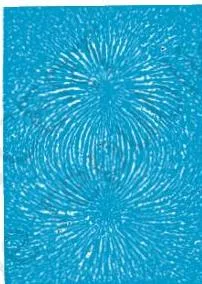
The iron-filing pattern of Figure 5.1 shows field lines leaving one pole, curving through space, and re-entering the other pole. Because the field lines are continuous, the magnet acts like a dipole, not like an isolated pair of charges.
\[ B_A = \frac{\mu_0}{4\pi}\frac{2m}{r^3} \]
Far axial field — field at a point on the axis, with \(r \gg l\) (NCERT, pp. 138, 140). The field points along \(\mathbf{m}\).
\[ \mathbf{B}_E = -\frac{\mu_0}{4\pi}\frac{\mathbf{m}}{r^3} \]
Far equatorial field — field at a point on the normal bisector, with \(r \gg l\). The minus sign means the field is opposite to \(\mathbf{m}\). At the same distance, the axial field is twice the equatorial field in magnitude.
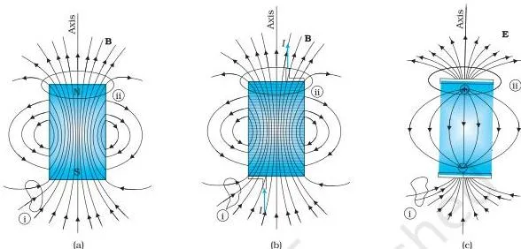
Figure 5.3(a) is the geometry used to derive the axial field of a finite solenoid; at large distances it reproduces the bar-magnet formula above. Figure 5.3(b) is the set-up behind the next group — a needle free to rotate in a uniform field.
The mapping between electric and magnetic dipoles (NCERT, p. 140) lets you reuse electric-dipole results directly:
| Quantity | Electrostatics | Magnetism |
|---|---|---|
| Dipole moment | \(\mathbf{p}\) | \(\mathbf{m}\) |
| Equatorial field (short dipole) | \(-\dfrac{\mathbf{p}}{4\pi\varepsilon_0 r^3}\) | \(-\dfrac{\mu_0 \mathbf{m}}{4\pi r^3}\) |
| Axial field (short dipole) | \(\dfrac{2\mathbf{p}}{4\pi\varepsilon_0 r^3}\) | \(\dfrac{\mu_0 2\mathbf{m}}{4\pi r^3}\) |
| Torque in an external field | \(\mathbf{p} \times \mathbf{E}\) | \(\mathbf{m} \times \mathbf{B}\) |
| Energy in an external field | \(-\mathbf{p}\cdot\mathbf{E}\) | \(-\mathbf{m}\cdot\mathbf{B}\) |
The Dipole in a Uniform Magnetic Field
\[ \boldsymbol{\tau} = \mathbf{m} \times \mathbf{B}, \qquad \tau = mB\sin\theta \]
Torque on the dipole (NCERT, p. 139). Here \(\theta\) is the angle between \(\mathbf{m}\) and \(\mathbf{B}\). In a uniform field the net force is zero, so only this torque acts.
\[ U_m = -\mathbf{m}\cdot\mathbf{B} = -mB\cos\theta \]
Magnetic potential energy, with the zero chosen at \(\theta = 90^\circ\) (NCERT, p. 139).
\[ U_{\min} = -mB \ (\theta = 0^\circ), \qquad U_{\max} = +mB \ (\theta = 180^\circ) \]
Energy is lowest when \(\mathbf{m}\) is parallel to \(\mathbf{B}\) (stable equilibrium) and highest when anti-parallel (unstable equilibrium). A released needle always swings toward \(\theta = 0^\circ\).
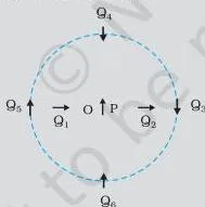
In Figure 5.4 (Example 5.2), needle Q is in stable equilibrium wherever \(\mathbf{m}_Q\) is parallel to the local field \(\mathbf{B}_p\), and in unstable equilibrium wherever it is anti-parallel (NCERT, p. 141).
Magnetism and Gauss’s Law
Flux through a small area element, then through the whole closed surface (NCERT, p. 142):
\[ \Delta\phi_B = \mathbf{B}\cdot\Delta\mathbf{S} \]
\[ \phi_B = \sum_{\text{all}} \mathbf{B}\cdot\Delta\mathbf{S} = 0 \]
Gauss’s law for magnetism: the net magnetic flux through any closed surface is zero. This is the direct consequence of the fact that isolated magnetic poles (monopoles) do not exist.
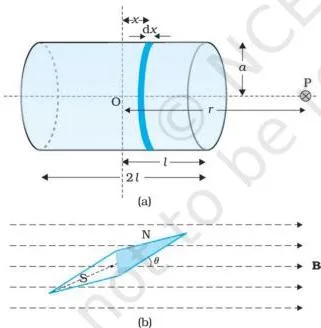
Figure 5.2 shows why the flux is always zero: magnetic field lines of a bar magnet and a solenoid form continuous closed loops, so as many lines leave any closed surface as enter it. The electric dipole (right) is different — its lines start on positive charge and end on negative charge.
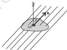
Figure 5.5 shows the building block: divide the closed surface into small vector area elements \(\Delta\mathbf{S}\), add \(\mathbf{B}\cdot\Delta\mathbf{S}\) over all of them, and the total is always zero.
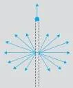
Figure 5.6 collects suspicious field-line drawings. Use the rules above as the test: field lines never cross, never start or end at a point, and every static magnetic field line must close on a current.
Magnetisation and Magnetic Intensity
Magnetisation is the net magnetic moment per unit volume of the sample (NCERT, p. 145):
\[ \mathbf{M} = \frac{\mathbf{m}_{\text{net}}}{V} \]
A long solenoid with \(n\) turns per unit length and current \(I\) produces (NCERT, p. 145):
\[ \mathbf{B}_0 = \mu_0 n I \]
With a material core, the total field is the solenoid field plus the material’s contribution:
\[ \mathbf{B} = \mathbf{B}_0 + \mathbf{B}_m, \qquad \mathbf{B}_m = \mu_0 \mathbf{M} \]
Magnetic intensity \(\mathbf{H}\) separates the external contribution from the material’s response (NCERT, p. 146):
\[ \mathbf{H} = \frac{\mathbf{B}}{\mu_0} – \mathbf{M}, \qquad \mathbf{B} = \mu_0(\mathbf{H} + \mathbf{M}) \]
For a long solenoid this reduces to \(H = nI\). Note that \(H\) comes only from the external source — it never picks up the material factor (Example 5.5, NCERT, p. 146).
For linear materials, magnetisation is proportional to magnetic intensity (NCERT, p. 146):
\[ \mathbf{M} = \chi \mathbf{H} \]
Combining the two relations gives the field inside the material in three equivalent forms:
\[ \mathbf{B} = \mu_0(1+\chi)\mathbf{H} = \mu_0\mu_r\mathbf{H} = \mu\mathbf{H} \]
\[ \mu_r = 1+\chi, \qquad \mu = \mu_0\mu_r = \mu_0(1+\chi) \]
Only one of \(\chi\), \(\mu_r\) and \(\mu\) is independent; given one, the other two follow (NCERT, p. 146).
Magnetic Properties of Materials
The sign and size of \(\chi\) decide how a material responds to an external field (NCERT, p. 147):
| Quantity | Diamagnetic | Paramagnetic | Ferromagnetic |
|---|---|---|---|
| \(\chi\) | \(-1 \le \chi \lt 0\) | \(0 \lt \chi \lt \varepsilon\) | \(\chi \gg 1\) |
| \(\mu_r\) | \(0 \le \mu_r \lt 1\) | \(1 \lt \mu_r \lt 1+\varepsilon\) | \(\mu_r \gg 1\) |
| \(\mu\) | \(\mu \lt \mu_0\) | \(\mu \gt \mu_0\) | \(\mu \gg \mu_0\) |
\(\varepsilon\) is a small positive number. Since \(\mu_r = 1 + \chi\), a diamagnet has \(\mu_r \lt 1\), a paramagnet just above 1, and a ferromagnet very large.
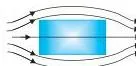
Figure 5.7(a) shows why \(\mu \lt \mu_0\) for a diamagnet: the material expels field lines. In the paramagnetic case (Figure 5.7(b)) the opposite happens — field lines concentrate inside, so the field is slightly enhanced (NCERT, p. 147).
A superconductor is a perfect diamagnet (the Meissner effect), with (NCERT, p. 148):
\[ \chi = -1, \qquad \mu_r = 0, \qquad \mu = 0 \]
What Each Symbol Means
Units follow the physical-quantities table at the end of the chapter (NCERT).
| Symbol | What it means | Unit (nature) |
|---|---|---|
| \(\mathbf{B}\) | Total magnetic field (magnetic induction) in a material; also the field of the bar magnet in the field formulas | Vector; tesla (T), \(10^4\ \text{G} = 1\ \text{T}\) |
| \(\mathbf{B}_0\) | Magnetic field inside a long solenoid with no core | Vector; T |
| \(\mathbf{B}_m\) | Field contributed by the magnetisation of the material core | Vector; T |
| \(\mathbf{m}\) | Magnetic moment of the magnet or dipole | Vector; \(\text{A m}^2\) (also written \(\text{J T}^{-1}\)) |
| \(\mathbf{m}_{\text{net}}\) | Net magnetic moment of the whole sample | Vector; \(\text{A m}^2\) |
| \(r\) | Distance from the centre of the magnet to the field point | m |
| \(l\) | Length (size) of the magnet | m |
| \(\theta\) | Angle between \(\mathbf{m}\) and \(\mathbf{B}\) | Angle (dimensionless; degrees or radians) |
| \(\boldsymbol{\tau}\) | Torque on the dipole | Vector; N m |
| \(U_m\) | Magnetic potential energy of the dipole | Scalar; J |
| \(\phi_B\) | Magnetic flux through a surface | Scalar; Wb, \(1\ \text{Wb} = 1\ \text{T m}^2\) |
| \(\Delta\mathbf{S}\) | Small vector area element of a surface | Vector; \(\text{m}^2\) |
| \(\mathbf{M}\) | Magnetisation: net magnetic moment per unit volume | Vector; \(\text{A m}^{-1}\) |
| \(V\) | Volume of the sample | \(\text{m}^3\) |
| \(n\) | Number of turns per unit length of a solenoid | \(\text{m}^{-1}\) |
| \(I\) | Current in the solenoid | A |
| \(\mathbf{H}\) | Magnetic intensity (field due to external sources) | Vector; \(\text{A m}^{-1}\) |
| \(\chi\) | Magnetic susceptibility | Scalar; dimensionless |
| \(\mu_r\) | Relative magnetic permeability | Scalar; dimensionless |
| \(\mu\) | Magnetic permeability of the material | Scalar; \(\text{T m A}^{-1}\) |
| \(\mu_0\) | Permeability of free space, \(4\pi \times 10^{-7}\ \text{T m A}^{-1}\) | Scalar; \(\text{T m A}^{-1}\) |
| \(\varepsilon\) | Small positive number used to quantify paramagnetic materials | Dimensionless |
When to Use Each Formula
| Formula | Use it when… | Condition to check |
|---|---|---|
| \(B_A = \dfrac{\mu_0}{4\pi}\dfrac{2m}{r^3}\) | You need the field at a point far from the magnet on its axis. | \(r \gg l\); point on the axial line. |
| \(\mathbf{B}_E = -\dfrac{\mu_0\mathbf{m}}{4\pi r^3}\) | You need the field far from the magnet on its normal bisector (equatorial line). | \(r \gg l\); field points opposite to \(\mathbf{m}\). |
| \(\boldsymbol{\tau} = \mathbf{m} \times \mathbf{B}\) | Torque on a needle, bar magnet or current loop in a uniform external field. | Field uniform; \(\theta\) is the angle between \(\mathbf{m}\) and \(\mathbf{B}\). |
| \(U_m = -\mathbf{m}\cdot\mathbf{B}\) | Potential energy of a dipole, or work done to rotate it between two orientations. | Zero of energy fixed at \(\theta = 90^\circ\). |
| \(\phi_B = \sum \mathbf{B}\cdot\Delta\mathbf{S} = 0\) | Net flux through any closed Gaussian surface; also a test of whether a field-line sketch is possible. | Any closed surface; no magnetic monopoles. |
| \(\mathbf{M} = \mathbf{m}_{\text{net}}/V\) | Magnetisation from a sample’s net moment and volume. | Bulk sample with a net moment. |
| \(\mathbf{H} = \dfrac{\mathbf{B}}{\mu_0} – \mathbf{M}\) | Converting between total field, magnetic intensity and magnetisation inside a material. | Material core present. |
| \(H = nI\) | Magnetic intensity inside a long solenoid. | \(n\) is turns per metre, not total turns. |
| \(\mathbf{M} = \chi\mathbf{H}\) | Magnetisation of a linear material in response to the applied intensity. | Linear material; \(\chi\) small for dia- and paramagnets. |
| \(\mathbf{B} = \mu_0\mu_r\mathbf{H}\) | Field inside a material-filled solenoid when \(\mu_r\) or \(\chi\) is given. | Core fills the region where \(\mathbf{B}\) is measured. |
Worked Examples
Example 1 — Torque and potential energy of a dipole
Step 1: A short bar magnet of moment \(m = 0.60\ \text{A m}^2\) is placed in a uniform field \(B = 0.40\ \text{T}\), with its axis at \(30^\circ\) to the field.
Pick the torque formula \(\tau = mB\sin\theta\).
\[ \tau = (0.60)(0.40)\sin 30^\circ = 0.24 \times 0.5 = 0.12\ \text{N m} \]
Step 2: Potential energy from \(U_m = -mB\cos\theta\).
\[ U_m = -(0.60)(0.40)\cos 30^\circ = -0.24 \times 0.866 \approx -0.21\ \text{J} \]
Final answer: \(\tau = 0.12\ \text{N m}\), \(U_m \approx -0.21\ \text{J}\).
Example 2 — Finding the magnetic moment from the axial field
Step 1: A short bar magnet produces \(B = 5.0 \times 10^{-5}\ \text{T}\) at a point 0.20 m from its centre on its axis.
Here \(r \gg l\), so use \(B_A = \dfrac{\mu_0}{4\pi}\dfrac{2m}{r^3}\) and solve for \(m\).
\[ m = \frac{B_A r^3}{2(\mu_0/4\pi)}, \qquad \frac{\mu_0}{4\pi} = 10^{-7}\ \text{T m A}^{-1} \]
Step 2: Substitute \(B_A = 5.0 \times 10^{-5}\ \text{T}\) and \(r = 0.20\ \text{m}\).
\[ m = \frac{(5.0 \times 10^{-5})(0.20)^3}{2 \times 10^{-7}} = \frac{5.0 \times 10^{-5} \times 8.0 \times 10^{-3}}{2.0 \times 10^{-7}} = 2.0\ \text{A m}^2 \]
Final answer: \(m = 2.0\ \text{A m}^2\).
Example 3 — Solenoid with a material core: H, B and M
Step 1: A long solenoid has \(n = 2000\) turns per metre and carries \(I = 1.5\ \text{A}\).
Its core has \(\mu_r = 300\).
Magnetic intensity comes only from the external source: \(H = nI\).
\[ H = 2000 \times 1.5 = 3.0 \times 10^3\ \text{A m}^{-1} \]
Step 2: Total field using the alternative form \(B = \mu_0\mu_r H\).
\[ B = (4\pi \times 10^{-7})(300)(3.0 \times 10^3) = 36\pi \times 10^{-2} \approx 1.1\ \text{T} \]
Step 3: Magnetisation from \(M = (\mu_r – 1)H\).
\[ M = (300 – 1)(3.0 \times 10^3) = 299 \times 3.0 \times 10^3 = 8.97 \times 10^5\ \text{A m}^{-1} \]
Final answer: \(H = 3.0 \times 10^3\ \text{A m}^{-1}\), \(B \approx 1.1\ \text{T}\), \(M = 8.97 \times 10^5\ \text{A m}^{-1}\). Check: \(B = \mu_0(H+M)\) gives the same \(B\).
Common Mistakes to Avoid
| Mistake | Correct rule | How to check your answer |
|---|---|---|
| Using the axial formula on the equatorial line, or forgetting the factor 2 and the minus sign. | The axis carries \(2m\) and is positive; the equator carries \(m\) alone and points opposite to \(\mathbf{m}\). | For the same \(r\), the axial magnitude is exactly twice the equatorial magnitude. |
| Applying the far-field dipole formulas when the point is close to the magnet. | \(B_A\) and \(\mathbf{B}_E\) are valid only for \(r \gg l\). | Compare \(r\) with the magnet’s length; near the magnet these formulas are only rough approximations. |
| Reversing stable and unstable equilibrium — treating \(U = +mB\) as the minimum. | \(U = -mB\cos\theta\): minimum \(-mB\) at \(\theta = 0^\circ\) (parallel, stable); maximum \(+mB\) at \(180^\circ\) (anti-parallel, unstable). | A released dipole swings toward \(\theta = 0^\circ\), the position of lowest energy — never the other way. |
| Treating \(H\) and \(B\) as the same field and quoting \(H\) in tesla. | \(\mathbf{H}\) is magnetic intensity in \(\text{A m}^{-1}\); \(\mathbf{B} = \mu_0(\mathbf{H}+\mathbf{M})\) is the total field in T. Only in free space is \(\mathbf{B} = \mu_0\mathbf{H}\). | Check units: a field in \(\text{A m}^{-1}\) is \(H\) or \(M\), never \(B\). |
| Putting the total number of turns \(N\) into \(H = nI\). | \(n\) is turns per metre: \(n = N/L\) for a solenoid of length \(L\). | \(H = nI\) must come out in \(\text{A m}^{-1}\); if it comes out in A, you used \(N\). |
| Expecting a non-zero net magnetic flux through a closed surface (electric-style thinking). | Gauss’s law for magnetism: \(\phi_B = 0\) for every closed surface, because magnetic monopoles do not exist. | Count field lines entering and leaving the surface; the two must balance. |
Frequently Asked Questions
Where is the magnetic potential energy zero, minimum and maximum?
By choice of the integration constant, the zero of \(U_m\) is at \(\theta = 90^\circ\) (\(\mathbf{m}\) perpendicular to \(\mathbf{B}\)). The energy is minimum, \(-mB\), at \(\theta = 0^\circ\) and maximum, \(+mB\), at \(\theta = 180^\circ\) (NCERT, p. 139).
Why is the axial field twice the equatorial field at the same distance?
For a short dipole, \(B_A = \dfrac{\mu_0}{4\pi}\dfrac{2m}{r^3}\) while \(B_E = \dfrac{\mu_0}{4\pi}\dfrac{m}{r^3}\), so \(B_A = 2B_E\) in magnitude. This mirrors the electric-dipole results in Table 5.1 (NCERT, p. 140).
What is the difference between B, H and M?
\(\mathbf{B}\) is the total magnetic field (tesla), \(\mathbf{H}\) is the magnetic intensity produced by external sources (\(\text{A m}^{-1}\)), and \(\mathbf{M}\) is the magnetisation of the material (\(\text{A m}^{-1}\)). They are related by \(\mathbf{B} = \mu_0(\mathbf{H}+\mathbf{M})\). In free space \(\mathbf{M} = 0\), so \(\mathbf{B} = \mu_0\mathbf{H}\) (NCERT, p. 146).
What are the susceptibility ranges for diamagnetic, paramagnetic and ferromagnetic materials?
Diamagnetic: \(-1 \le \chi \lt 0\), field reduced. Paramagnetic: \(0 \lt \chi \lt \varepsilon\), field slightly enhanced. Ferromagnetic: \(\chi \gg 1\), strong response. A superconductor is a perfect diamagnet with \(\chi = -1\) (NCERT, pp. 147–148).
All equations follow the Rationalised NCERT Class 12 Physics Part I textbook, chapter 5 (Magnetism and Matter). The official chapter PDF is leph105.pdf on the NCERT website. For formula sheets of other classes, see the Physics formulas main index.
Reference: NCERT Class 12 Physics textbook, chapter Magnetism and Matter.
Explore Class 12 Physics Formulas
More for this chapter:
Class 12 Physics on LearnCBSE:
Related chapters: