This page collects the Current Electricity Class 12 formulas from NCERT Physics Part I, Chapter 3. It covers steady and instantaneous current, Ohm’s law and resistance, drift velocity and mobility, resistivity and its temperature dependence, electrical power, cells (emf and internal resistance), Kirchhoff’s rules and the Wheatstone bridge.
Each formula is grouped by topic, with the meaning and unit of every symbol, guidance on when each formula is used, three worked examples and chapter-specific common mistakes. This sheet is part of the Class 12 Physics formulas collection; it is a lookup sheet, so derivations are kept to a line each.
Formulas at a Glance
| Purpose (what you are finding) | Formula |
|---|---|
| Steady current from charge and time | \( I = \dfrac{q}{t} \) |
| Instantaneous (time-varying) current | \( I = \lim_{\Delta t \to 0}\dfrac{\Delta Q}{\Delta t} \) |
| Current from drift speed and electron density | \( I = neAv_d \) |
| Voltage across a conductor (Ohm’s law) | \( V = IR \) |
| Resistance of a wire from its dimensions | \( R = \rho\dfrac{l}{A} \) |
| Local form of Ohm’s law inside a material | \( \mathbf{j} = \sigma\mathbf{E} \), \( \sigma = \dfrac{1}{\rho} \) |
| Drift velocity of electrons in a field | \( \mathbf{v}_d = -\dfrac{e\mathbf{E}}{m}\tau \) |
| Conductivity and resistivity from the electron model | \( \sigma = \dfrac{ne^2\tau}{m} \), \( \rho = \dfrac{m}{ne^2\tau} \) |
| Mobility of charge carriers | \( \mu = \dfrac{|\mathbf{v}_d|}{E} = \dfrac{e\tau}{m} \) |
| Resistivity at temperature \( T \) | \( \rho_T = \rho_0[1 + \alpha(T – T_0)] \) |
| Power dissipated in a resistor | \( P = VI = I^2R = \dfrac{V^2}{R} \) |
| Power lost in transmission cables (derived from \( P = VI \)) | \( P_c = I^2R_c = \dfrac{P^2R_c}{V^2} \) |
| Terminal voltage of a cell delivering current | \( V = \varepsilon – Ir \) |
| Current from a cell with internal resistance \( r \) | \( I = \dfrac{\varepsilon}{R + r} \), \( V = IR = \dfrac{\varepsilon R}{R + r} \) |
| Maximum current from a cell (short-circuit, derived by setting \( R = 0 \)) | \( I_{\max} = \dfrac{\varepsilon}{r} \) |
| Cells in series (an opposing cell enters with a negative emf) | \( \varepsilon_{eq} = \sum\varepsilon_i \), \( r_{eq} = \sum r_i \) |
| Cells in parallel | \( \dfrac{1}{r_{eq}} = \sum\dfrac{1}{r_i} \), \( \dfrac{\varepsilon_{eq}}{r_{eq}} = \sum\dfrac{\varepsilon_i}{r_i} \) |
| Kirchhoff’s junction rule — currents at a junction | \( \sum I_{\text{in}} = \sum I_{\text{out}} \) |
| Kirchhoff’s loop rule — potential changes around a loop | \( \sum \Delta V = 0 \) |
| Wheatstone bridge balance (null deflection) | \( \dfrac{R_1}{R_2} = \dfrac{R_3}{R_4} \); unknown \( R_4 = R_3\dfrac{R_2}{R_1} \) |
All Formulas, Grouped by Topic
The formula inventory below groups the equations of this chapter by the NCERT section in which each appears. Verify any equation against the official NCERT Physics Part I textbook (Chapter 3, Current Electricity).
Electric Current
For a steady current, the net charge \( q \) crossing an area in time \( t \) defines the current:
\[ I = \frac{q}{t} \]
If the current varies with time, use the instantaneous value — the limit of the charge-to-time ratio as the interval shrinks to zero:
\[ I(t) = \lim_{\Delta t \to 0} \frac{\Delta Q}{\Delta t} \]
In a metal, the current is carried by electrons drifting with speed \( v_d \) (NCERT, p. 86):
\[ I = neAv_d \]
Current is a scalar: through an area \( \Delta\mathbf{S} \) it is the scalar product \( I = \mathbf{j}\cdot\Delta\mathbf{S} \), even though it is drawn with an arrow (NCERT, p. 104).
Ohm’s Law
Ohm’s law states that the current through a conductor is proportional to the potential difference across its ends (NCERT, p. 83):
\[ V = RI \]
\( R \) is the resistance of the conductor, with \( 1\ \Omega = 1\ \text{V A}^{-1} \). The law holds because in a metal the drift speed is proportional to the field, so doubling the voltage doubles the drift speed and hence the current.
Resistance depends on the conductor’s dimensions (NCERT, p. 83):
\[ R = \rho\frac{l}{A} \]
Doubling the length doubles \( R \); halving the cross-sectional area also doubles \( R \), because the current then has half as many parallel paths. The resistivity \( \rho \) is a material property, independent of size.

The local form of Ohm’s law relates the electric field and current density at a point inside the material (NCERT, p. 84):
\[ \mathbf{E} = \rho\mathbf{j}, \qquad \mathbf{j} = \sigma\mathbf{E}, \qquad \sigma = \frac{1}{\rho} \]
Current density is also written \( \mathbf{j} = nq\mathbf{v}_d \), where \( q \) is the charge on each carrier — for electrons \( q = -e \) (NCERT, p. 103).
Drift of Electrons and the Origin of Resistivity
Electrons accelerate under the field but keep colliding with the fixed ions; the average velocity is the steady drift velocity (NCERT, p. 86):
\[ \mathbf{v}_d = -\frac{e\mathbf{E}}{m}\tau \]
The minus sign shows electrons drift opposite to the field. The relaxation time \( \tau \) is the average time between successive collisions — each collision randomises the direction of motion, so the electrons settle at a constant average speed instead of accelerating forever.
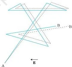
The same model reproduces Ohm’s law and predicts the conductivity (NCERT, p. 86):
\[ \sigma = \frac{ne^2\tau}{m}, \qquad \rho = \frac{1}{\sigma} = \frac{m}{ne^2\tau} \]
Resistivity rises when collisions become more frequent (\( \tau \) falls) and falls when more free electrons are available (\( n \) rises).
Mobility
Mobility is the magnitude of drift velocity per unit electric field (NCERT, p. 88):
\[ \mu = \frac{|\mathbf{v}_d|}{E} = \frac{e\tau}{m} \]
Mobility is always positive and is measured in \( \text{m}^2\ \text{V}^{-1}\ \text{s}^{-1} \).
Temperature Dependence of Resistivity
Over a limited temperature range, resistivity changes almost linearly with temperature (NCERT, p. 90):
\[ \rho_T = \rho_0[1 + \alpha(T – T_0)] \]
\( \alpha \) is the temperature coefficient of resistivity. For metals \( \alpha \gt 0 \): heating makes collisions more frequent, reducing \( \tau \) and raising \( \rho \). For semiconductors, resistivity decreases with temperature because \( n \) rises.
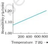
Electrical Energy and Power
The power dissipated when current \( I \) flows through a potential difference \( V \) (NCERT, p. 92):
\[ P = VI \]
Using Ohm’s law \( V = IR \) gives three equivalent forms:
\[ P = VI = I^2R = \frac{V^2}{R} \]
Charges lose potential energy as they cross the conductor, and collisions transfer that energy to the atoms — which is why the conductor heats up.
Power wasted in transmission cables of resistance \( R_c \), when a device of power \( P \) is driven at voltage \( V \) (NCERT, p. 92):
\[ P_c = I^2R_c = \frac{P^2R_c}{V^2} \]
This is why power is transmitted at very high voltage: for a fixed delivered power \( P \), the loss falls as \( 1/V^2 \).
Cells, EMF and Internal Resistance
A cell is the device that maintains a steady current. As Figure 3.1 shows, drifting electrons would neutralise the separated charges and stop the current unless the source continuously replenishes them.

Emf \( \varepsilon \) is the open-circuit potential difference between the electrodes. While the cell delivers current \( I \), its internal resistance \( r \) drops a voltage \( Ir \), so the terminal voltage is less than the emf (NCERT, p. 94):
\[ V = \varepsilon – Ir \]
With an external resistance \( R \), the circuit current and external voltage are:
\[ I = \frac{\varepsilon}{R + r}, \qquad V = IR = \frac{\varepsilon R}{R + r} \]
The maximum current is drawn when \( R = 0 \): \( I_{\max} = \varepsilon / r \) (NCERT, p. 94).
Cells in Series and in Parallel
Series combination, same polarity (NCERT, p. 95–96):
\[ \varepsilon_{eq} = \varepsilon_1 + \varepsilon_2 + \dots, \qquad r_{eq} = r_1 + r_2 + \dots \]
A cell whose current leaves its negative electrode enters the sum with a negative sign; two opposing cells give \( \varepsilon_{eq} = \varepsilon_1 – \varepsilon_2 \) with \( \varepsilon_1 \gt \varepsilon_2 \) (NCERT, p. 95–96).
Parallel combination of \( n \) cells (NCERT, p. 96):
\[ \frac{1}{r_{eq}} = \frac{1}{r_1} + \dots + \frac{1}{r_n}, \qquad \frac{\varepsilon_{eq}}{r_{eq}} = \frac{\varepsilon_1}{r_1} + \dots + \frac{\varepsilon_n}{r_n} \]
For just two cells these give \( \varepsilon_{eq} = (\varepsilon_1 r_2 + \varepsilon_2 r_1)/(r_1 + r_2) \) and \( r_{eq} = r_1 r_2/(r_1 + r_2) \).
Kirchhoff’s Rules
Junction rule — at any junction, the sum of the currents entering equals the sum of the currents leaving (NCERT, p. 97):
\[ \sum I_{\text{in}} = \sum I_{\text{out}} \]
Loop rule — the algebraic sum of changes in potential around any closed loop is zero:
\[ \sum \Delta V = 0 \]
The junction rule follows from conservation of charge: with steady currents, charge cannot pile up at a junction. The loop rule follows from conservation of energy: returning to the starting point after one loop, the potential must come back to its original value.
Wheatstone Bridge
The Wheatstone bridge is four resistors \( R_1, R_2, R_3, R_4 \) with a source across one diagonal and a galvanometer across the other. At balance, no current flows through the galvanometer and the balance condition is (NCERT, p. 101):
\[ \frac{R_2}{R_1} = \frac{R_4}{R_3} \]
The same condition is often written \( \frac{R_1}{R_2} = \frac{R_3}{R_4} \) (NCERT, p. 104). With three known resistances, the unknown fourth is:
\[ R_4 = R_3\frac{R_2}{R_1} \]
Why it works: with \( I_g = 0 \), the junction rule gives \( I_1 = I_3 \) and \( I_2 = I_4 \); applying the loop rule to loops ADBA and CBDC forces both \( I_1/I_2 = R_2/R_1 \) and \( I_1/I_2 = R_4/R_3 \), hence the two ratios must be equal (NCERT, p. 101).
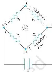
What Each Symbol Means
The table gives the meaning and SI unit of every symbol used on this sheet, with the dimensional formula from the NCERT summary table (NCERT, p. 104).
| Symbol | What it means | SI unit | Dimensions |
|---|---|---|---|
| \( I \) | Electric current — net charge crossing a cross-section per unit time | ampere (A) | [A] |
| \( q,\ Q \) | Electric charge crossing an area | coulomb (C) | [T A] |
| \( t,\ \Delta t \) | Time interval | second (s) | [T] |
| \( V \) | Potential difference between two points of a conductor | volt (V) | [M L² T⁻³ A⁻¹] |
| \( R \) | Resistance of a conductor | ohm (\( \Omega \)) | [M L² T⁻³ A⁻²] |
| \( \rho \) | Resistivity — a material property, independent of size | ohm metre (\( \Omega\ \text{m} \)) | [M L³ T⁻³ A⁻²] |
| \( \sigma \) | Conductivity, equal to \( 1/\rho \) | siemens per metre (\( \text{S}\ \text{m}^{-1} \)) | [M⁻¹ L⁻³ T³ A²] |
| \( l \) | Length of the conductor | metre (m) | [L] |
| \( A \) | Cross-sectional area | square metre (\( \text{m}^2 \)) | [L²] |
| \( \mathbf{E} \) | Electric field inside the conductor | volt per metre (\( \text{V}\ \text{m}^{-1} \)) | [M L T⁻³ A⁻¹] |
| \( \mathbf{j} \) | Current density — current per unit area normal to the flow | ampere per square metre (\( \text{A}\ \text{m}^{-2} \)) | [L⁻² A] |
| \( n \) | Number density of free electrons (carriers per unit volume) | per cubic metre (\( \text{m}^{-3} \)) | [L⁻³] |
| \( e \) | Magnitude of the electronic charge | coulomb (C) | [T A] |
| \( \mathbf{v}_d \) | Drift velocity — average velocity of electrons under the field | metre per second (\( \text{m}\ \text{s}^{-1} \)) | [L T⁻¹] |
| \( \tau \) | Relaxation time — average time between successive collisions | second (s) | [T] |
| \( \mu \) | Mobility — drift speed per unit electric field | square metre per volt-second (\( \text{m}^2\ \text{V}^{-1}\ \text{s}^{-1} \)) | [M⁻¹ T² A] |
| \( \alpha \) | Temperature coefficient of resistivity | per kelvin (\( \text{K}^{-1} \)) | [K⁻¹] |
| \( T,\ T_0 \) | Temperature and reference temperature | kelvin (K) or degree Celsius | [K] |
| \( P \) | Electric power dissipated | watt (W) | [M L² T⁻³] |
| \( \varepsilon \) | Emf of a cell — open-circuit terminal potential difference | volt (V) | [M L² T⁻³ A⁻¹] |
| \( r \) | Internal resistance of a cell | ohm (\( \Omega \)) | [M L² T⁻³ A⁻²] |
When to Use Each Formula
This table gives guidance on when each formula is used and the condition that must hold for it to be valid.
| Use this when… | Formula | Condition |
|---|---|---|
| Net charge crosses an area at a steady rate | \( I = q/t \) | Steady current |
| Current changes with time | \( I = dQ/dt \) | Instantaneous value |
| Current from electron drift in a metal | \( I = neAv_d \) | \( n \) is the free-electron density |
| Potential difference across a conductor | \( V = IR \) | Defines \( R \) for any device; Ohm’s law adds \( R \) independent of \( V \) |
| Resistance of a uniform wire | \( R = \rho l/A \) | Uniform cross-section, homogeneous material |
| Field and current density inside a conductor | \( \mathbf{j} = \sigma\mathbf{E} \) | \( \sigma \) independent of \( \mathbf{E} \) (ohmic material) |
| Resistivity at another temperature | \( \rho_T = \rho_0[1+\alpha(T-T_0)] \) | Limited temperature range, linear behaviour |
| Power dissipated in a resistor | \( P = I^2R = V^2/R \) | Use \( I^2R \) when current is known, \( V^2/R \) when voltage is known |
| Power lost in transmission cables | \( P_c = P^2R_c/V^2 \) | Fixed delivered power \( P \); loss falls as \( V \) rises |
| Terminal voltage while a cell supplies current | \( V = \varepsilon – Ir \) | Current leaves the positive terminal; in open circuit \( V = \varepsilon \) |
| Circuit current with a real cell | \( I = \varepsilon/(R+r) \) | Cell of emf \( \varepsilon \), internal resistance \( r \) |
| Combining cells in series | \( \varepsilon_{eq} = \sum\varepsilon_i \), \( r_{eq} = \sum r_i \) | Same polarity; an opposing cell contributes \( -\varepsilon_i \) |
| Combining cells in parallel | \( 1/r_{eq} = \sum 1/r_i \), \( \varepsilon_{eq}/r_{eq} = \sum \varepsilon_i/r_i \) | Positive terminals joined, negative terminals joined |
| Currents meeting at a junction | \( \sum I_{\text{in}} = \sum I_{\text{out}} \) | Steady currents, no charge accumulation |
| Potential changes around a closed loop | \( \sum \Delta V = 0 \) | Include each cell with the correct sign |
| Finding an unknown resistance in a bridge | \( R_4 = R_3R_2/R_1 \) | Galvanometer null deflection (balanced bridge) |
Worked Examples
Three worked examples using original numbers show how to select the formula, substitute with units, and check the answer.
Worked Example 1: Finding Drift Speed from the Current
Given: a copper wire of cross-sectional area \( 2.0 \times 10^{-6}\ \text{m}^2 \) carries a steady current of \( 4.0\ \text{A} \).
The free-electron number density of copper is \( 8.5 \times 10^{28}\ \text{m}^{-3} \).
Step 1 — select the formula: current and drift speed are connected by \( I = neAv_d \), so \[ v_d = \frac{I}{neA} \]
Step 2 — substitute with units: \( e = 1.6 \times 10^{-19}\ \text{C} \), \[ v_d = \frac{4.0}{(8.5 \times 10^{28})(1.6 \times 10^{-19})(2.0 \times 10^{-6})} = \frac{4.0}{2.72 \times 10^{4}} = 1.47 \times 10^{-4}\ \text{m s}^{-1} \]
Final answer: \( v_d \approx 1.5 \times 10^{-4}\ \text{m s}^{-1} \), about 0.15 mm per second. Unit check: \( \text{A}/(\text{m}^{-3}\cdot\text{C}\cdot\text{m}^2) = \text{m s}^{-1} \). ✓
Worked Example 2: Working Backwards to Find the Temperature Coefficient
Given: a wire has resistance \( 40.0\ \Omega \) at \( 20^\circ\text{C} \).
In an oven at \( 120^\circ\text{C} \) its resistance rises to \( 58.0\ \Omega \).
Step 1 — select the formula: \( R_T = R_0[1 + \alpha(T – T_0)] \) with \( R_0 \) measured at \( T_0 \).
Rearrange for \( \alpha \):
\[ \alpha = \frac{R_T/R_0 – 1}{T – T_0} \]
Step 2 — substitute:
\[ \alpha = \frac{58.0/40.0 – 1}{120 – 20} = \frac{0.45}{100} = 4.5 \times 10^{-3}\ {}^\circ\text{C}^{-1} \]
Final answer: \( \alpha = 4.5 \times 10^{-3}\ {}^\circ\text{C}^{-1} \). The positive sign is consistent with metallic behaviour — resistance rises with temperature.
Worked Example 3: A Real Cell — Current and Terminal Voltage
Given: a battery of emf \( 6.0\ \text{V} \) and internal resistance \( 0.50\ \Omega \) is connected across a \( 5.5\ \Omega \) resistor.
Step 1 — select the formula: the total resistance in the circuit is \( R + r \), so \[ I = \frac{\varepsilon}{R + r} = \frac{6.0}{5.5 + 0.50} = \frac{6.0}{6.0} = 1.0\ \text{A} \]
Step 2 — terminal voltage: compute it two ways and confirm they agree — as the voltage across \( R \), and from the cell’s own terminal relation:
\[ V = IR = 1.0 \times 5.5 = 5.5\ \text{V} \]
\[ V = \varepsilon – Ir = 6.0 – 1.0(0.50) = 5.5\ \text{V} \]
Final answer: current \( 1.0\ \text{A} \); terminal voltage \( 5.5\ \text{V} \) — \( 0.5\ \text{V} \) less than the emf, dropped inside the battery across its internal resistance.
Common Mistakes to Avoid
These are chapter-specific errors in applying the formulas above — each with the correct rule and a quick check to run on your own answer.
| Mistake | Correct rule | How to check your answer |
|---|---|---|
| Treating \( V = IR \) as the whole of Ohm’s law for any device. | \( V = IR \) defines resistance and applies to any conductor. Ohm’s law is the stronger statement that \( R \) is independent of \( V \), so the I–V graph is a straight line (NCERT, p. 104). A diode has a value of \( V/I \) at every point but does not obey Ohm’s law. | Double the voltage: does the current double? Only if it does is the device ohmic. |
| Using the emf \( \varepsilon \) as the voltage across the load. | \( \varepsilon \) is the open-circuit terminal voltage. While the cell supplies current, \( V = \varepsilon – Ir \), so the terminal voltage is smaller than the emf (NCERT, p. 94). | Compute \( V \) twice — as \( IR \) and as \( \varepsilon – Ir \). The two must match. |
| Giving a cell the wrong sign in a loop when current leaves its negative electrode. | A cell whose current leaves the negative terminal contributes \( -\varepsilon \). Two opposing cells in series give \( \varepsilon_{eq} = \varepsilon_1 – \varepsilon_2 \) with \( \varepsilon_1 \gt \varepsilon_2 \) (NCERT, p. 95–96). | Walk once around the loop in your chosen direction; the first electrode you enter fixes the sign of that cell. |
| Writing resistivity in ohm instead of ohm-metre. | From \( R = \rho l/A \), \( \rho = RA/l \), so the unit is \( \Omega\ \text{m} \). Conductivity \( \sigma = 1/\rho \) is in \( \text{S}\ \text{m}^{-1} \). | Units in \( R = \rho l/A \): \( \Omega\ \text{m} \times \text{m}/\text{m}^2 = \Omega \). ✓ |
| For cells in parallel, averaging the emfs directly. | Use \( 1/r_{eq} = \sum 1/r_i \) and \( \varepsilon_{eq}/r_{eq} = \sum \varepsilon_i/r_i \). The equivalent emf is a weighted average; the simple average is valid only when the cells are identical (NCERT, p. 96). | Two identical cells in parallel: \( r_{eq} = r/2 \), \( \varepsilon_{eq} = \varepsilon \) — not \( 2\varepsilon \) and not \( \varepsilon/2 \). |
Frequently Asked Questions
Is V = IR the same as Ohm’s law?
No. \( V = IR \) defines the resistance of any conductor and can be applied even to devices that do not obey Ohm’s law. Ohm’s law is the additional statement that I is proportional to V — that R is independent of V — so the I–V graph is a straight line (NCERT, p. 104).
Why is emf called a force if it is not a force?
The name is historical. Emf is a potential difference: the voltage between the terminals of a cell in open circuit, measured in volts, not newtons (NCERT, p. 94).
When can internal resistance be ignored?
When the current is small enough that \( \varepsilon \gg Ir \), the terminal voltage is effectively \( \varepsilon \) (NCERT, p. 94). If a problem gives \( r \), use \( V = \varepsilon – Ir \) and \( I = \varepsilon/(R + r) \).
Why is the drift speed so small if the current is large?
Because the electron number density is enormous — of the order of \( 10^{29}\ \text{m}^{-3} \) (NCERT, p. 88). A vast number of carriers, each drifting slowly, still transports a large net charge across any cross-section every second.
Need a formula from another chapter? Browse the physics formula index.
Reference: NCERT Class 12 Physics textbook, chapter Current Electricity.
Explore Class 12 Physics Formulas
More for this chapter:
Class 12 Physics on LearnCBSE:
Related chapters: