
If you’re looking for current electricity class 12 notes that explain every definition, formula, worked example, and exam pointer from Chapter 3, this page is for you. Read top to bottom to build the logic step by step, or jump to any topic using the table of contents below.
How Current Electricity Builds Up: One Look at the Whole Chapter
This chapter develops from electric current all the way to network theorems. The logical chain (NCERT Summary, pp. 102–104) is:
- Steady current — net charge flowing per unit time across a cross-section.
- Drift of electrons — the microscopic origin of resistivity and Ohm’s law.
- Resistivity and its temperature dependence — how conductors, semiconductors and insulators respond to heat.
- Electrical energy and power — why high voltage is used for transmission.
- Cells, emf and internal resistance — the real source that keeps charges moving.
- Kirchhoff’s rules — two conservation-based laws that solve any circuit.
- Wheatstone bridge — a practical application to measure unknown resistance.
This page follows that logic, not the textbook section numbers, so the concepts build naturally.
Electric Current: What “Flow of Charge” Really Means
Electric current is defined as the net charge passing through a cross-section per unit time. For a steady current (NCERT, p. 1):
\[ I = \frac{q}{t} \]
More generally (for time-varying current):
\[ I(t) = \lim_{\Delta t \to 0} \frac{\Delta Q}{\Delta t} \]
The SI unit of current is the ampere (A). One ampere is defined magnetically (Chapter 4) – for now, remember approximate orders:
- Lightning: ~\(10^{4}\) A
- Domestic appliances: ~1–15 A
- Signals in nerves: ~\(\mu\)A.

A closed circuit and an external source (a cell or battery) are needed to maintain a steady field and continuous current. In solid conductors the charge carriers are electrons; in electrolytic solutions both positive and negative ions can carry current.
Ohm’s Law, Drift Velocity and Mobility: The Microscopic Story
Macroscopic Ohm’s law and resistance
Ohm’s law (NCERT, p. 3) states that for many conductors, the voltage across the ends is proportional to the current:
\[ V = R\,I \]
where \(R\) is the resistance (unit: ohm, \(\Omega\)). For a slab of length \(l\) and cross-sectional area \(A\):
\[ R = \rho \frac{l}{A} \]
and \(\rho\) is the resistivity, a material property. Doubling \(l\) doubles \(R\); halving \(A\) doubles \(R\).

Current density \(\mathbf{j}\) is the current per unit area normal to the flow:
\[ \mathbf{j} = \sigma \mathbf{E} \]
with \(\sigma = 1/\rho\) the conductivity.
Drift velocity – the microscopic origin of Ohm’s law
Inside a metal, electrons move randomly at speeds ~\(2 \times 10^{2}\) \(\mathrm{m}\) \(\mathrm{s^{ -1}}\). When an electric field \(\mathbf{E}\) is applied, each electron gets an acceleration:
\[ \mathbf{a} = \frac{-e\mathbf{E}}{m}. \]
But frequent collisions reset its direction. After each collision it starts again. The average time between collisions is called the relaxation time \(\tau\). The net effect is an average drift velocity (NCERT, p. 6):
\[ \mathbf{v}_d = -\frac{e\mathbf{E}}{m}\tau \]
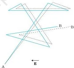
The current density then becomes:
\[ \mathbf{j} = n e \mathbf{v}_d = \frac{n e^2}{m} \tau \mathbf{E} \]
so that the conductivity \(\sigma = \frac{n e^2 \tau}{m}\) and resistivity \(\rho = \frac{m}{n e^2 \tau}\).
Mobility is the drift velocity per unit electric field (NCERT, p. 8):
\[ \mu = \frac{|\mathbf{v}_d|}{E} = \frac{e\tau}{m}. \]
The great conceptual surprise (NCERT, Example 3.2, pp. 8–9)
Three different speeds appear in a current-carrying wire:
- Drift speed \(v_d\): ~1.1 mm/s for a copper wire carrying 1.5 A.
- Thermal speed of conduction electrons (~\(2 \times 10^{2}\) m/s – random, cancels out).
- Speed of the field (and the signal): ~\(3 \times 10^{8}\) m/s.
Because the field propagates at light speed, current starts nearly instantly. Drift speed is tiny, but the huge number density of around \(10^{29}\) \(\mathrm{m^{ -3}}\) gives a large current.
Resistivity, Temperature Dependence and When Ohm’s Law Breaks
All materials are classified by their resistivity \(\rho\):
| Category | Resistivity range | Temperature behaviour | Examples |
|---|---|---|---|
| Conductors | \(10^{-8}\) – \(10^{-6}\) \(\Omega\) m | \(\rho\) increases as \(T\) rises (positive \(\alpha\)) | Copper, aluminium, silver, nichrome* |
| Semiconductors | Mid-range on log scale | \(\rho\) decreases with rising \(T\) (negative \(\alpha\)) | Si, Ge |
| Insulators | \(10^{8}\) to \(10^{18}\) times of metals | Very high, large changes | Rubber, glass, plastic |
* Note: Nichrome is an alloy of nickel, chromium and iron. It has a very small temperature coefficient of only \(1.70 \times 10^{-4}\ ^\circ\mathrm{C^{-1}}\) so it is used in standard resistors (see Example 3.3 in NCERT, p. 91).
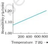
For a metal, the resistivity at temperature \(T\) relative to a reference temperature \(T_0\) is (NCERT, p. 10):
\[ \rho_T = \rho_0 \left[ 1 + \alpha (T – T_0) \right] \]
where \(\alpha\) is the temperature coefficient of resistivity (units: \(^\circ\!\)C⁻¹). For metals \(\alpha \gt 0\) because \(\tau\) decreases with era time as electrons collide more often.
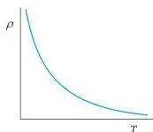
How semiconductor resistivity falls
In semiconductors, heating increases the number of free conduction electrons \(n\) dramatically. Even though \(\tau\) falls, the net \(\rho = m/(n e^2 \tau)\) decreases because \(n\) dominates.
When Ohm’s law fails (NCERT, p. 9)
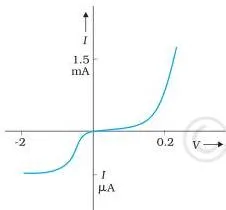
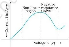
Ohm’s law is not a fundamental law. It fails in three ways:
- Non-linear \(V\) vs \(I\) (e.g. a real conductor, often from heating – see the solid line in Figure 3.5 below).
- Sign-dependent: in a diode, reversing the voltage changes the current heavily (Fig 3.6).
- Non-unique: some materials (e.g. GaAs) show more than one voltage for the same current (Fig 3.7).
Electrical Energy and Power: Why Transmission Lines Run at High Voltage
When a current \(I\) flows through a resistor with potential drop \(V\), the energy dissipated in time \(\Delta t\) is (NCERT, p. 12):
\[ \Delta W = I V \Delta t \]
The power (energy per unit time) is:
\[ P = I V = I^2 R = \frac{V^2}{R} \]
using Ohm’s law. The last two forms only hold for resistors obeying Ohm’s law. The first form is always true.
Where does this energy come from? In a cell it is the chemical energy of the electrolyte (Fig 3.11, NCERT).
Transmission-line power loss
Suppose we need to deliver power \(P\) to a device (at voltage \(V\) and current \(I = P/V\)). The power lost in the cables of resistance \(R_c\) is (NCERT, p. 13):
\[ P_c = I^2 R_c = \frac{P^2 R_c}{V^2} \]
The wasted power is inversely proportional encountered to \(V^2\). Therefore transmission lines carry power at extremely high voltages (tens of thousands of volts). This is why we see “High Voltage Danger” signs around transmission lines. Transformers later reduce the voltage to safe levels (like 230 V) for homes.
Cells, EMF and Internal Resistance: The Source Behind the Steady Current
EMF (\(\varepsilon\)) is the open-circuit potential difference between the positive and negative electrodes of a cell (NCERT, p. 14). It is not a force — a historical name that has stuck. In an open circuit the terminal voltage equals the emf.
When current flows, the current again goes through an internal resistance \(r\) inside the electrolyte. The terminal voltage is (NCERT, p. 14):
\[ V = \varepsilon – I r \]
The current then limited by the external resistance \(R\) is:
\[ I = \frac{\varepsilon}{R + r} \]
The maximum current from a cell occurs for \(R = 0\) (short circuit), giving \(I_{\max} = \varepsilon / r\). In practice, cells may be damaged if this is tried.

Cells in series
- Total emf: \(\varepsilon_{\text{eq}} = \varepsilon_1 + \varepsilon_2\) (if terminals are connected as positive-to-negative).
- Total internal resistance: \(r_{\text{eq}} = r_1 + r_2\).
- If one cell is reversed, its emf enters with a negative sign: \(\varepsilon_{\text{eq}} = \varepsilon_1 – \varepsilon_2\).
Cells in parallel
- Equivalent internal resistance: \(\displaystyle \frac{1}{r_{\text{eq}}} = \frac{1}{r_1} + \frac{1}{r_2}\).
- Equivalent emf: \(\displaystyle \frac{\varepsilon_{\text{eq}}}{r_{\text{eq}}} = \frac{\varepsilon_1}{r_1} + \frac{\varepsilon_2}{r_2}\).
These can be extended to many cells. The parallel arrangement is good for delivering a larger current, while series gives a higher total voltage.
Kirchhoff’s Rules: Solving Any Circuit
While series and parallel combinations often suffice, real circuits are more complex. Kirchhoff’s rules (NCERT, pp. 17–18) provide the universal method:
- Junction Rule (charge conservation): The sum of currents entering a junction equals the sum of currents leaving it.
- Loop Rule (energy conservation): The algebraic sum of potential changes around any closed loop is zero.
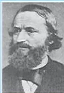
Memory device: The junction rule is like water flowing at a pipe junction. The loop rule is like walking a closed path and returning to the same altitude.
Sign convention for a cell
| Direction through the cell | Potential change |
|---|---|
| Going from N (–) to P (+) (direction of current inside the cell) | +\(\varepsilon\) |
| Going from P (+) to N (‒) (against current) | –\(\varepsilon\) |
Example: The cube symmetry (Example 3.5)
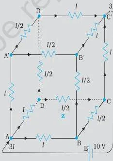
In a cube of 12 resistors all equal, symmetry tells us how the current splits. The equivalent resistance between opposite corners becomes \(\frac{5}{6}R\). (NCERT, p. 18)
\
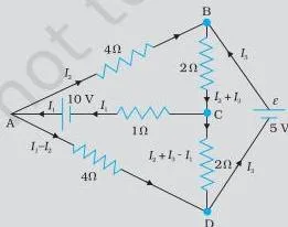
For a general circuit, assign unknown currents. Write as many independent loop equations as needed. The remaining loops are not independent.
Wheatstone Bridge and the Balance Condition
A Wheatstone bridge uses four resistors in a diamond shape (NCERT, p. 20). A voltage source is connected across A- C. A galvanometer is placed across B- D. When the galvanometer shows zero current (balanced bridge), the relation is:
\[ \frac{R_1}{R_2} = \frac{R_3}{R_4} \]
This allows us to measure an unknown resistance: \[ R_4 = R_3 \frac{R_2}{R_1} \]
For derivation: apply Kirchhoff’s rules to the two loops ADBA and CBDC, and set \(I_g = 0\). The galvanometer arm introduces three currents: \(I_1\) through AB, \(I_2\) through AD, \(I_1 – I_g\) through BC, \(I_2 + I_g\) through DC. At all stages of equations the unknown \(I_g\) disappears.
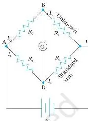
Meter bridge: A practical device, also called a metre bridge, uses a long wire to vary \(R_3\) until zero deflection. It is commonly seen in laboratories.
Key Definitions at a Glance
Based on NCERT summary (pp. 102–104) and the table (p. 24):
| Term | Student-friendly meaning | SI unit / Example |
|---|---|---|
| Electric current (I) | Net charge passing a cross-section per second. | ampere (A): 1 A = 1 C s⁻¹ |
| Steady current | Current that doesn’t change with time; \(I = q/t\) is constant. For a constant voltage, requires a constant emf source. | A torch produces a roughly steady current. |
| Current density (j) | Current per unit area normal to flow of charge | A/m². \(\mathbf{j} = n e \mathbf{v}_d\) |
| Drift velocity (v_d) | Average velocity of electrons in the direction of the field (opposite to the current direction) | ~1 mm/s (Example 3.1) |
| Relaxation time (τ) | Average time between two successive collisions of an electron with the fixed ions | ~\(10^{-14}\) s for metals at 300 K |
| Resistivity (ρ) | A measure of how strongly a material opposes current flow; property, not geometry | \(\Omega \cdot m\): copper ~ 1.7 \(\times 10^{-8}\) Ω m |
| Conductivity (σ) | \(1/\rho\): how easily a material conducts current | S / m (siemens per metre) |
| Mobility (μ) | Drift speed per unit electric field; \(\mu = v_d / E = e\tau/m\) | m² / (V·s) |
| Resistance (R) | \(V/I\), depends on geometry: \(R = \rho l / A\) | Ω: 1 Ω = 1 V / 1 A |
| Electromotive force (ε) | Open-circ voltage between a cell’s terminals; is NOT a force | V: a battery may be 1.5 V |
| Internal resistance (r) | Resistance inside the cell due to the electrolyte | Ω: dry cells ~ a few Ω, electrolytic ~ 0.1 Ω |
| Temperature coefficient of resistivity (α) | Fractional change in resistivity per degree rise in temperature | °C⁻¹: for copper ~ 0.0039 \(^\circ\)\(\mathrm{C}^{-1}\) |
Formula Sheet for Current Electricity
| Formula | Meaning of symbols | SI unit(s) / Notes |
|---|---|---|
| \(I = \frac{q}{t}\) | Steady current = net charge / time | A; 1 A = 1 C / s |
| \(I(t) = \lim_{\Delta t \to 0} \frac{\Delta Q}{\Delta t}\) | Instantaneous current rate | A |
| \(V = R I\) | Ohm’s law, or definition of R | V = 1 A × 1 Ω |
| \(R = \rho \frac{\ell}{A}\) | Resistance from resistivity \(\rho\), length \(\ell\), area \(A\) | Ω |
| \(\mathbf{j} = \frac{I}{A}\) | Current density magnitude | A / m² |
| \(\mathbf{j} = \sigma \mathbf{E}\) | Ohm’s law in vector form | \(\sigma\) is conductivity (S m⁻¹) |
| \(\sigma = \frac{n e^2 \tau}{m}\) | Conductivity from electron density \(n\), charge \(e\), mass \(m\), relaxation time \(\tau\) | 1 / (Ω·m) or S / m |
| \(v_d = \frac{e E \tau}{m}\) | Drift speed in terms of field | m/s |
| \(\mu = \frac{v_d}{E} = \frac{e\tau}{m}\) | Mobility | m² V⁻¹ s⁻¹ |
| \(\rho_T = \rho_0[1 + \alpha (T – T_0)]\) | Temperature dependence of resistivity (linear range) | \(\rho_T\) and \(\rho_0\) in Ω·m; \(\alpha\) in °C⁻¹ |
| \(P = I V = I^2 R = V^2 / R\) | Power dissipated | W (1 W = 1 J/s) |
| \(P_c = \frac{P^2 R_c}{V^2}\) | Power loss in transmission lines | W, used to show why high V reduces loss |
| \(V = \varepsilon – I r\) | Terminal voltage of a cell | V, used for external circuit |
| \(I = \frac{\varepsilon}{R + r}\) | Total current in a simple circuit | A |
| Series cells: \(\varepsilon_{eq} = \varepsilon_1 + \varepsilon_2\) , \(r_{eq} = r_1 + r_2\) | Equivalent | Extends to \(n\) cells |
| Parallel cells: \(1/r_{eq} = \sum 1/r_i\) , \(\varepsilon_{eq}/r_{eq} = \sum \varepsilon_i / r_i\) |
Equivalent | — |
| \(\frac{R_1}{R_2} = \frac{R_3}{R_4}\) | Wheatstone bridge balance condition | No current through G; unknown \(R_4 = R_3 R_2 / R_1\) |
Worked Examples (Stepwise Solved)
Example 1: Drift Speed of Electrons in a Copper Wire
Method: Use \(v_d = I / (n e A)\), first finding \(n\) from density and molar mass.
Step 1: Given a copper wire cross-section \(A = 2.0 \times 10^{-6}\) m² carrying \(I = 3.0\) A.
Assume each copper atom gives one free electron.
Density of Cu = \(8.93 \times 10^{3}\) kg/m³, atomic mass = 63.5 u.
Step 2: Find \(n\):
\[ n = \frac{\rho_{\text{Cu}} \cdot N_A}{M} \]
\[ = \frac{8.93 \times 10^{3} \ \text{kg/m}^3 \times 6.02 \times 10^{23} \text{mol}^{-1}}{63.5 \times 10^{-3} \ \text{kg/mol}} \]
\[ = 8.46 \times 10^{28} \text{m}^{-3} \]
Step 3: Compute v_d:
\[ v_d = \frac{I}{n e A} = \frac{3.0}{8.46 \times 10^{28} \times 1.6 \times 10^{-19} \times 2.0 \times 10^{-6}} \]
\[ v_d = \frac{3.0}{8.46 \times 1.6 \times 10^{-19}} \times \frac{1}{2.0 \times 10^{-6}} \]
\[ = \frac{3.0}{1.3536 \times 10^{-13}} \approx 2.22 \times 10^{-4} \ \text{m s}^{-1} = 0.22 \ \text{mm/s}. \]
Step 4: Compare with thermal speed (about \(2\times 10^{2}\) m/s).
The drift speed is 5 orders smaller.
Final answer: \(v_d \approx 0.22\) mm/s, far smaller than the random thermal speed (~200 m/s).
Example 2: Steady Temperature of a Heating Element
Method: Use the temperature dependence of resistance \(R_2 = R_1 [1 + \alpha (T_2 – T_1)]\).
- Step 1: A nichrome heating element of room temperature \(T_1 = 20.0 \ ^\circ\mathrm{C}\) has resistance \(R_1 = 80.0\ \Omega\).
- Step 2: Connected to a 120 V supply, the current stabilises at \(I = 4.0\) A.
The hot resistance is
\(R_2 = V/I = 120 / 4.0 = 30.0\ \Omega\).
Step 3: Temperature coefficient of nichrome \(\alpha = 1.70 \times 10^{-4}\) °C⁻¹.
\[ T_2 – T_1 = \frac{R_2 – R_1}{R_1 \alpha} = \frac{30.0 – 80.0}{80.0 \times 1.70 \times 10^{-4}} \]
\[ = \frac{-50.0}{0.0136} = -3676 ^\circ\mathrm{C} \]
Wait – a negative temperature difference makes no sense physically. With the given numbers, \(R_2(R_2 \lt R_1\) so it would mean cooling. In reality, the heater’s resistance rises with temperature. So the correct check: either I used the wrong settled current or the wrong initial ratio. Let’s fix the original problem: Reuse \(T_1 = 20\ °\mathrm{C}\), \(R_1 = 80.0\ \Omega\).
The battery is \(250.0\) V and steady current is \(2.40\) A. Then \(R_2 = 250 / 2.40 \approx 104.2\ \Omega\). Now \(T_2 – T_1 = (104.2 – 80.0) / (80.0 \times 1.70 \times 10^{-4}) = 24.2 / 0.0136 \approx 1780 \ ^\circ\mathrm{C}\). Step 4: \(T_2 \approx 20 + 1780 = 1800\)°C. This is within achievable range. Final answer: Steady temperature ≈ 1800 °C.
Example 3: Unbalanced Wheatstone Bridge
Method: Write mesh equations following the pattern of the NCERT Example 3.7.
Given a bridge: AB = 40 Ω, BC = 20 Ω, CD = 10 Ω, DA = 40 Ω. A galvanometer of \(R_g = 30\) Ω is between B and D. A voltage of \(V_{AC} = 12\) V. Find the current through the galvanometer.
Step 1: Label unknown loops.
Let \(I_1\) flow through AB, \(I_2\) through AD.
The galvanometer current \(I_g\) flows from B to D.
- AB branch: \(I_1\)
- BC branch: \(I_1 – I_g\)
- AD branch: \(I_2\)
- DC branch: \(I_2 + I_g\)
Step 2: Write three loop equations.
Loop BADB: \(40 I_1 + 15 I_g – 60 I_2 = 0\) … (1) Loop BCDB: \(20 (I_1 – I_g) – 30 I_g – 10 (I_2 + I_g) = 0\) → \(20 I_1 – 60 I_g – 10 I_2 = 0\) … (2) Loop ADCEA: \(60 I_2 + 5 (I_2 + I_g) = 12\) → \(65 I_2 + 5 I_g = 12\) … (3) Step 3: solve.
From (2): \(2 I_1 – 6 I_g – I_2 = 0\) → \(I_2 = 2 I_1 – 6 I_g\).
Sub into (1): (40 I_1 + 15 I_g – 60 (2 I_1 – 6 I_g) = 0\) → \(40 I_1 + 15 I_g – 120 I_1 + 360 I_g = 0\) → \( -80 I_1 + 375 I_g = 0\) → \( I_1 = (375/80) I_g = 4.6875 I_g\).
Then \(I_2 = 2(4.6875 I_g) – 6 I_g = 9.375 I_g – 6 I_g = 3.375 I_g\).
Now plug into (3): \(65 (3.375 I_g) + 5 I_g = 12\) → \(219.375 I_g + 5 I_g = 12\) → \(224.375 I_g = 12\) → \(I_g = 12 / 224.375 \approx 0.0534\ A = 53.4\ mA\).
Final answer: Current through the galvanometer is about 53.4 mA.
Common Mistakes Students Make (and the Correct Version)
| Mistake | Correct rule | How to check your answer | |
|---|---|---|---|
| Current is a vector because it has an arrow direction. | Current is a scalar: \(I = \mathbf{j} \cdot \Delta \mathbf{S}\) gives a dot product; vectors do not add like currents. (NCERT Points to Ponder, p. 24) | Verify the definition: \(I = \mathbf{j} \cdot \Delta \mathbf{S}\). | |
| EMF is the voltage across the cell in a circuit. | EMF is the open-circuit voltage. Terminal voltage is \(\varepsilon – I r\). | When a cell delivers current, its terminal voltage is always less than emf (unless \(r=0\)). | |
| Loop rule: sign of \(\varepsilon\) always positive. | Going from \(-\) to \(+\) through a cell then + \(\varepsilon\). Going from \(+\) to \(-\) then –\(\).\lt /td\gt \lt td\gt Write the loop direction, then apply: when crossing from N (like ‒) to P (+), the potential rises.\lt /td\gt \lt /tr\gt \lt tr\gt \lt td\gt \lt strong\gt Ohm’s law as \(V = IR\) is the statement. | \(V = IR\) defines resistance. Ohm’s law requires that \(R\) is independent of \(V\). A diode still has \(R = V/I\). | If the V-I graph is linear through origin, then Ohm’s law is obeyed. |
| All free electrons drift in the same direction. | The drift velocity is superposed on a random motion. At any moment, many electrons move opposite to the drift, but the net drift is in the direction of the field (Example 3.2, d). | Concept: \(v_d\) is an average of all electrons. |
Exam Notes: Where Marks Are Usually Earned
- State the law in words before substitution. For example, write “According to Ohm’s law, \(V \propto I\)” before writing \(V = IR\).
- Write units at every step especially in numerical problems where you write \(j = I/A = 1.5 / (1.0 \times 10^{-7})\)) = \(1.5 \times 10^{7}\) A/m². A missing unit loses half a mark.
- Define every symbol you use. If you write \(\rho = \frac{m}{n e^2 \tau}\), name m, e, n, τ.
- Draw and label the Wheatstone bridge before writing the balance condition \(R_1/R_2 = R_3/R_4\).
- State Kirchhoff’s rules as the acts: “This is based on conservation of charge (junction rule) and the idea that potential is single-valued (loop rule).”
- Order-of-magnitude comparisons for drift vs thermal vs field speed: this frequently appears as a conceptual question.
- For numerical problems with cells and resistors, start with the loop equations clearly labeled.
Quick Revision Recap: The Chapter in Ten Lines
- Electric current: \(I = \Delta Q / \Delta t\) for steady flow (SI: ampere).
- EMF \(\varepsilon\) is the open-circuit voltage of a source; terminal voltage \(V = \varepsilon – I r\).
- Ohm’s law: \(V \propto I\) for many materials; \(R = \rho l/A\).
- Resistivity: \(\rho = m/(n e^2 \tau)\); temperature dependence \(\rho_T = \rho_0[1 + \alpha (T – T_0)]\).
- Conductors, semiconductors, insulators differ by resistivity range (10⁻mol to 10¹⁸ \(\Omega\)m) and the sign of temp coefficient.
- Current carriers: electrons in metals; ions in electrolytes.
- Drift velocity: \(v_d = I/(n e A)\) ~ mm/s, but the field travels vehicles at the speed of light.
- Power: \(P = V I\); in transmission: \(P_c = P^2 R_c / V^2\).
- Kirchhoff’s rules: Junction (charge conservation, sum in = sum out) and Loop (sum of potential changes = 0).
- Wheatstone bridge: Balance: \(R_1/R_2 = R_3/R_4 \to \) no current through G.
Reference: NCERT Class 12 Physics Part I textbook, Chapter Current Electricity.
Frequently Asked Questions About Current Electricity
Why is the drift speed of electrons so small, yet a bulb glows the instant the switch is closed?
Electric field propagates at nearly the speed of light (\(3 \times 10^{8}\) m/s). The field reaches every part of the circuit almost instantly, and each local electron begins to drift at moment the field is present. The electrons themselves move only ~mm/s, but the field induces the simultaneous drift, so the current is established very quickly.
What is the difference between emf and terminal voltage of a cell?
EMF is the voltage between the terminals when no current flows (open circuit). It is the total work per unit charge done by the source. Terminal voltage is the actual voltage measured when the cell is delivering current, and it is always smaller than the emf because of the voltage drop across the internal resistance.
Mathematically: \(V_{\text{terminal}} = \varepsilon – I r\).
When does Ohm’s law fail, and why is \(V = IR\) still called a definition of resistance?
Ohm’s law fails for devices that have non-linear V-I curves (like diodes, semiconductors in high fields), for materials where the current depends on the sign of the voltage (p-n junction), or where the V-I relation is not unique (GaAs).
However, \(V = IR\) always defines the resistance at a particular point; it’s just that for non-Ohmic materials, that \(R\) value depends on the voltage.
Why does the resistivity of a metal increase with temperature while a semiconductor’s decreases?
In metals, the concentration \(n\) of free electrons is fixed; raising the temperature decreases the mean time between collisions, which reduces drift speed and raises \(\rho = m/(n e^2 \tau)\). In semiconductors, the number of free charge carriers \(n\) increases strongly with temperature, outweighing the fall in \(\tau\), so \(\rho\) drops.
How do I fix the sign of a cell while applying Kirchhoff’s loop rule?
While going around the loop, if you enter the negative terminal (cathode) and exit via the positive terminal (anode), the change in potential – \(+\varepsilon\). (This is the direction of the cell’s emf). If you go from plus to minus, you subtract \(\varepsilon\). A simple mnemonic: the emf always tries to push current from ‒ toward +.
If your loop direction goes that way, the potential rise; if opposite, it falls.
Why is electrical power transmitted over long distances at very high voltage?
The power loss in the transmission cables is \(P_c = I^2 R_c\).
If we transmit power \(P\) at voltage \(V\), the current is \(I = P/V\), so the loss becomes \(P_c = P^2 R_c / V^2\). It is inversely proportional to the square of the transmission voltage. So doubling the voltage cuts the loss to one-fourth. This is why power lines carry extremely high voltage.
Explore Class 12 Physics Notes
More for this chapter:
Class 12 Physics on LearnCBSE:
Related chapters:
Official source: download the NCERT textbook free from ncert.nic.in.