
This page collects the linear programming class 12 formulas you need when revising Chapter 12: the objective function \( Z = ax + by \), the constraint inequalities, the non-negative restrictions \( x \geq 0,\ y \geq 0 \), and the Corner Point Method with its bounded and unbounded checks.
Each formula is grouped by the textbook sub-topic it comes from, with a symbol table, when-to-use guidance, and worked examples using fresh numbers. For the full explanations and derivations, see the Class 12 Maths formulas hub; this sheet keeps only what you need at a glance.
Formulas at a Glance
The table below lists every formula and decision rule on this page. Symbols are explained in the next section.
| Purpose (what you are finding) | Formula |
|---|---|
| Objective function — the linear expression to be maximised or minimised | \( Z = ax + by \) |
| Non-negative restrictions on the decision variables | \( x \geq 0,\ \ y \geq 0 \) |
| Complete problem statement — maximise or minimise Z subject to all constraints | \( \text{Maximise or minimise } Z = ax + by \text{ subject to linear constraints and } x \geq 0,\ y \geq 0 \) |
| Value of Z at a corner point (direct substitution into the objective function) | \( Z_i = ax_i + by_i \) at vertex \( (x_i,\ y_i) \) |
| Bounded region — largest and smallest corner values are the optimum (Theorem 2) | \( M = \max Z, \quad m = \min Z \) when \( R \) is bounded |
| Unbounded region — a maximum exists only if this open half-plane misses the region | \( ax + by \gt M \) has no point in common with \( R \) |
| Unbounded region — a minimum exists only if this open half-plane misses the region | \( ax + by \lt m \) has no point in common with \( R \) |
| Multiple optimal solutions — when two corner points give the same optimum | Every point of the segment joining them gives the same \( Z \) |
All Formulas, Grouped by Topic
Mathematical Formulation of the Problem
A linear programming problem has one linear objective function, a set of linear constraints, and non-negative variables. The objective function is \( Z = ax + by \), where \( a \) and \( b \) are constants; the complete problem maximises or minimises it subject to the constraints and \( x \geq 0,\ y \geq 0 \) (NCERT, p. 397).
\[ Z = ax + by \]
The decision variables are non-negative:
\[ x \geq 0, \quad y \geq 0 \]
The furniture-dealer problem of the textbook shows how a word problem becomes this form (NCERT, p. 396). With \( x \) tables and \( y \) chairs, the formulation is:
\[ 2500x + 500y \leq 50000 \quad \text{(investment constraint)} \]
\[ 5x + y \leq 100 \quad \text{(after dividing by 500)} \]
\[ x + y \leq 60 \quad \text{(storage constraint)} \]
\[ Z = 250x + 75y \quad \text{(profit to be maximised)} \]
Every constraint keeps its inequality sign, the variables stay non-negative, and the objective adds the per-unit profits into one linear sum.
Graphical Method: Corner Point Method
The feasible region is the common region of all constraints including \( x \geq 0,\ y \geq 0 \); it is always a convex polygon (NCERT, p. 398). Every point inside or on it is a feasible solution, so the search for the optimum happens only on this region.
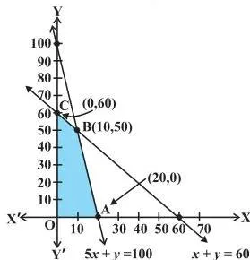
The Corner Point Method (NCERT, p. 399) then works in three steps.
- Graph every constraint and shade the feasible region. Find its corner points (vertices) by inspection or by solving the two boundary-line equations whose lines meet at the vertex.
- Evaluate the objective function at every corner point: \( Z_i = ax_i + by_i \) at \( (x_i,\ y_i) \). Let \( M \) be the largest and \( m \) the smallest of these values.
- Apply the decision rule:
- If the feasible region is bounded, \( M \) is the maximum and \( m \) is the minimum of \( Z \).
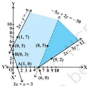
- If the region is unbounded, \( M \) is the maximum only when the open half-plane \( ax + by \gt M \) has no point in common with the region; otherwise no maximum exists. Similarly, \( m \) is the minimum only when the open half-plane \( ax + by \lt m \) has no point in common with the region; otherwise no minimum exists.
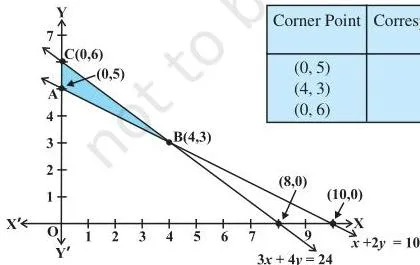
Bounded vs unbounded: a feasible region is bounded if it can be enclosed within a circle; otherwise it is unbounded and extends indefinitely in some direction (NCERT, p. 399).
When the region is bounded, as in the shaded region ABC below, the corner values give both extrema directly.
When the region is unbounded, as below, the half-plane check decides whether the corner value is a true optimum.
Theorems That Justify the Corner Point Method
Theorem 1: If \( Z = ax + by \) has an optimal value — maximum or minimum — subject to the constraints, that optimal value must occur at a corner point (vertex) of the feasible region.
Theorem 2: If the feasible region \( R \) is bounded, \( Z \) has both a maximum and a minimum on \( R \), and each occurs at a corner point (NCERT, p. 398).
Unbounded remark: If \( R \) is unbounded, a maximum or a minimum may not exist; if one does exist, it must occur at a corner point (NCERT, p. 398).
Why the corner rule holds: \( Z \) is linear, so along any straight edge of the feasible region it rises or falls at a steady rate. Its extreme value on that edge is therefore at an endpoint — a vertex.
Multiple Optimal Solutions and No-Feasible-Region Cases
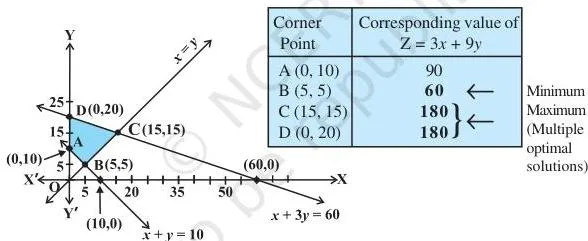
Multiple optimal solutions: if two corner points give the same maximum (or minimum) value of \( Z \), every point of the line segment joining them gives the same optimal value (NCERT, p. 402). In the region ABCD below, the maximum occurs at both corners C and D, so the whole segment CD is optimal.
No feasible solution: if the constraints contradict one another, no point satisfies all of them at once. The feasible region is empty and the problem has no feasible solution (NCERT, pp. 403–404), as the half-planes below show.
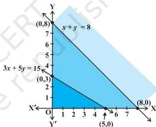
The feasible region is always a convex region, which is why the whole segment between two optimal corners stays inside the region (NCERT, p. 404).
What Each Symbol Means
Units matter in word problems: Z, M and m carry the units of the quantity being optimised, while a and b carry units per unit of the decision variable.
| Symbol | What it means | Unit / nature |
|---|---|---|
| \( Z \) | Value of the objective function — the quantity being maximised or minimised | The problem’s unit, e.g. rupees; a pure number in abstract problems |
| \( a, b \) | Constants in \( Z = ax + by \), usually profit or cost per unit of \( x \) and \( y \) | Per unit of the item (e.g. rupees per unit) |
| \( x, y \) | Decision variables — the quantities you choose | A count (number of items) |
| \( R \) | Feasible region — all points satisfying every constraint including \( x \geq 0,\ y \geq 0 \) | A region in the xy-plane |
| \( M \) | Largest value of \( Z \) among all corner points | Same as \( Z \) |
| \( m \) | Smallest value of \( Z \) among all corner points | Same as \( Z \) |
| \( (x_i, y_i) \) | The \( i \)-th corner point (vertex) of the feasible region | Coordinates in the xy-plane |
| corner point (vertex) | Intersection of two boundary lines of the feasible region | A point of the region |
When to Use Each Formula
| Formula or rule | Use it when … |
|---|---|
| \( Z = ax + by \) | A word problem gives per-unit profit or cost and asks for maximum profit or minimum cost — write this expression first. |
| \( x \geq 0,\ y \geq 0 \) | Always. Decision variables are counts, so the feasible region must stay in the first quadrant. |
| Corner Point Method | The problem says “solve graphically” — this chapter’s only method for two-variable LPPs. |
| Bounded region rule: \( M = \max Z,\ m = \min Z \) | The feasible region is enclosed on all sides; then no half-plane check is needed. |
| Unbounded region checks with \( ax + by \gt M \) or \( ax + by \lt m \) | The feasible region runs off indefinitely; do the check before claiming a maximum or minimum exists. |
| Multiple optimal segment rule | Two corner points give equal \( Z \) — the whole segment between them is optimal too. |
Worked Examples
Example 1: Maximise Z = 6x + 4y with a bounded region
Step 1: Write the constraints as lines and list the corner points.
Constraints: \( x + y \leq 40 \) and \( 3x + y \leq 60 \), with \( x \geq 0,\ y \geq 0 \). The lines \( x + y = 40 \) and \( 3x + y = 60 \) meet where \( 2x = 20 \), so \( x = 10,\ y = 30 \).
The corner points are \( (0,0) \), \( (20,0) \), \( (10,30) \) and \( (0,40) \). The point \( (40,0) \) is not a corner because \( 3(40) + 0 = 120 \gt 60 \).
Step 2: Evaluate \( Z = 6x + 4y \) at each corner.
\[ Z(0,0) = 0, \quad Z(20,0) = 120, \quad Z(10,30) = 6(10) + 4(30) = 180, \quad Z(0,40) = 160 \]
Step 3: The region is bounded, so the largest corner value is the maximum.
Final answer: \( Z = 180 \), the maximum, at the point \( (10, 30) \).
Example 2: Minimise Z = -3x + 2y with an unbounded region
Step 1: Graph the constraints and find the corner points.
Constraints: \( 2x – y \geq -4 \), \( x + y \geq 2 \), \( x – 2y \leq 4 \), \( x \geq 0,\ y \geq 0 \). The vertices are \( (0,2) \), \( (2,0) \), \( (4,0) \) and \( (0,4) \); each satisfies every constraint. The region is unbounded — it continues without limit to the right.
Step 2: Evaluate \( Z = -3x + 2y \) at the corners.
\[ Z(0,2) = 4, \quad Z(2,0) = -6, \quad Z(4,0) = -12, \quad Z(0,4) = 8 \]
The smallest corner value is \( m = -12 \) at \( (4,0) \).
Step 3: The region is unbounded, so test the open half-plane \( -3x + 2y \lt -12 \).
Take the feasible point \( (8,5) \): it satisfies all three constraints, and \( Z(8,5) = -24 + 10 = -14 \), which is less than \( -12 \). So the half-plane has points in common with the region, and \( -12 \) is not the minimum.
Final answer: \( Z \) has no minimum value subject to these constraints.
Example 3: Maximise Z = 3x + 3y with multiple optimal solutions
Step 1: List the corner points of the feasible region.
Constraints: \( x + y \leq 12 \), \( x + 2y \leq 16 \), \( x \geq 0,\ y \geq 0 \). Solving \( x + y = 12 \) and \( x + 2y = 16 \) gives \( (8,4) \); the other corners are \( (0,0) \), \( (12,0) \) and \( (0,8) \).
Step 2: Evaluate \( Z = 3x + 3y \) at each corner.
\[ Z(0,0) = 0, \quad Z(12,0) = 36, \quad Z(8,4) = 24 + 12 = 36, \quad Z(0,8) = 24 \]
The largest value \( M = 36 \) occurs at two corners, \( (12,0) \) and \( (8,4) \).
Step 3: When two corners give the same maximum, every point of the segment joining them gives the same value.
Check the midpoint \( (10,2) \): \( Z(10,2) = 30 + 6 = 36 \), and it satisfies both constraints.
Final answer: \( Z = 36 \), the maximum, attained at every point of the segment from \( (12,0) \) to \( (8,4) \).
Exercise 12.1 of the textbook has ten “solve graphically” problems in the same format: Q1–Q5 and Q9–Q10 ask for a single optimum, Q7 and Q8 ask for both the minimum and the maximum together, and Q6 asks you to show that the minimum occurs at more than two points.
A full-marks answer must show the shaded feasible region, list every corner point, evaluate Z at each corner, and state the optimal value with its point — running the half-plane check whenever the region is unbounded.
For more revision sheets on other chapters, browse the maths formulas directory.
Common Mistakes to Avoid
| Mistake | Correct rule | How to check your answer |
|---|---|---|
| Declaring the smallest corner value the minimum (or the largest the maximum) without checking whether the region is bounded. | For an unbounded region, \( m \) is the minimum only if the open half-plane \( ax + by \lt m \) has no point in common with the feasible region; likewise \( M \) with \( ax + by \gt M \). | Try to find one feasible point in that half-plane. If you can, the corner value is not the optimum. |
| Dropping the non-negative restrictions and using corner points outside the first quadrant. | The feasible region must satisfy \( x \geq 0,\ y \geq 0 \) as well as every constraint. | Every corner point you list must have both coordinates non-negative. |
| Using the closed half-plane \( \leq \) or \( \geq \) in the unbounded-region test. | The test uses the open half-plane — a strict inequality \( \lt \) or \( \gt \); boundary points do not count. | If only boundary points are common, the strict half-plane misses the region, so the corner value stands. |
| Writing a corner that lies on two boundary lines but fails another constraint. | A corner point must be inside the feasible region — it must satisfy every constraint, not just the two lines meeting there. | Substitute the point into all constraints before evaluating Z. |
| Treating two equal optimum values at two corners as a tie to break. | When two corners give the same optimum, every point of the segment joining them gives the same optimal value. | Test the midpoint of the segment — it must give the same Z. |
Frequently Asked Questions
Why does the optimum always occur at a corner point?
Because \( Z = ax + by \) is linear. Moving along any edge of the feasible region, Z changes at a steady rate, so its extreme value on that edge must be at an endpoint — a vertex. This is Theorem 1 of the chapter (NCERT, p. 398).
When do I need the half-plane check?
Only when the feasible region is unbounded. For a bounded region, Theorem 2 guarantees that M and m are the maximum and minimum directly. For an unbounded region, the open half-plane check with \( ax + by \gt M \) or \( ax + by \lt m \) decides whether the corner value is a genuine optimum (NCERT, p. 399).
Can a linear programming problem have no solution?
Yes, in two ways. The constraints may leave no common region, so there is no feasible solution at all (Fig 12.6). Or the region may be unbounded and the half-plane check shows the objective can keep improving without bound, so no finite maximum or minimum exists (Fig 12.5).
Two corner points give the same maximum value — what do I write as the answer?
State the maximum value and note that it is attained at both corner points and at every point of the line segment joining them (NCERT, p. 402).
Reference: NCERT Class 12 Mathematics textbook, chapter Linear Programming (Rationalised NCERT). Verify the formulas against the official textbook at ncert.nic.in.
Explore Class 12 Maths Formulas
More for this chapter:
Class 12 Maths on LearnCBSE:
Related chapters: