
Map projections are the answer to a practical problem: the globe shows the earth accurately, but you cannot fold it, carry it easily, or compare two regions on it.
These are the complete revision notes for Chapter 4, Map Projections of the NCERT Class 11 Geography textbook (Practical Work in Geography) — why projection is needed, the four bases of classification, every construction formula, three worked constructions with fresh numbers, and the properties, limitations and uses of each projection.
These notes follow the 2026-27 session. They sit inside the Class 11 Geography notes collection, and the other Class 11 notes are also available. To verify any figure or formula against the book, NCERT publishes the chapter as an official chapter PDF.
Why the Globe Cannot Be Flattened: The Need for Projection
The globe is the best model of the earth (NCERT, p. 35). It shows the shapes and sizes of continents and oceans accurately, and it also shows directions and distances correctly. But a globe is expensive, hard to carry, cannot show minor detail, and makes it difficult to compare two natural regions (p. 36).
This is why accurate large-scale maps on flat paper are needed.
On the globe, meridians are semi-circles and parallels are circles. When transferred to a plane, these lines become intersecting straight or curved lines (p. 35). If a flat sheet is stuck against a globe, it cannot coincide with the globe over a large surface without distortion.
Light placed at the centre of the globe produces a distorted picture away from the line or point of tangency, and distortion increases with distance from the tangential point (p. 36).
The deeper reason is that the globe is a non-developable surface — it cannot be flattened without shrinking, breaking or creasing (p. 38). So distortion is not a mistake in any one method; it is unavoidable when a non-developable curved surface is flattened. That is why every projection is a compromise.
Map projection is the method of transferring the graticule — the network of parallels and meridians (p. 35) — onto a plane surface. It is also defined as the study of the different methods tried for this transfer (p. 36).
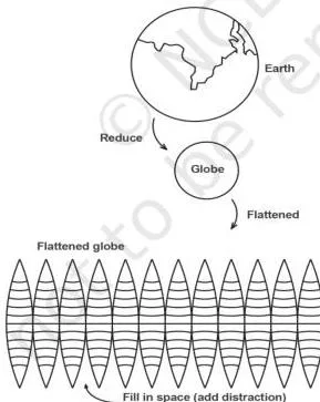
Figure 4.1 states the central problem of the chapter: flattening the globe distorts area, shape and directions. The rest of the chapter is a set of compromises — each projection sacrifices one property to save another.
Core Concepts: Graticule, Reduced Earth and Global Properties
Every construction in this chapter is built from the same four elements (NCERT, p. 37). Learn them in this order.
- Reduced earth: a model of the earth drawn on a reduced scale; it is roughly spheroid, with the polar diameter slightly less than the equatorial. The graticule is transferred on to this model (p. 37). The scale used is the Representative Fraction (R.F.) familiar from the chapter on map scale.
- Parallels of latitude: circles running round the globe parallel to the equator. They are not equal in length — they shrink from the equator to a point at each pole — and they are marked from 0° to 90° north and south (p. 37).
- Meridians of longitude: semi-circles running from pole to pole; two opposite meridians together make a full circle. There is no natural central meridian, so Greenwich (0°) is used as an arbitrary reference (p. 37).
- Global property: the four properties of the globe’s surface that a projection tries to preserve (p. 37).
The four global properties are: (i) distance between any two given points; (ii) shape of a region; (iii) size or area of a region; (iv) direction of one point bearing to another (p. 37). Remember them as ADDS — Area, Direction, Distance, Shape.
The punchline of the chapter is that no projection ADDS all four: no projection can maintain all these properties at once (p. 39).
How Map Projections Are Classified
A developable surface is one that can be flattened without shrinking, breaking or creasing; a non-developable surface cannot. A cylinder, a cone and a plane are developable; the globe is not (NCERT, p. 38).
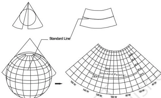
Figure 4.2 shows the idea behind one class of projections: a cone is wrapped round the globe, the graticule is projected on to it, and when the cone is cut open it gives a flat map (p. 38).
Projections are classified on four bases (pp. 37–40):
| Basis | Types | Key idea |
|---|---|---|
| Drawing technique | Perspective, non-perspective, mathematical/conventional | Perspective projections use a source of light; non-perspective ones do not; mathematical projections are derived from computation and formulae (pp. 37–38). |
| Developable surface | Cylindrical, conical, zenithal; each subdivided into normal, oblique and polar | A cylinder, cone or plane is wrapped around or touches the globe; its position gives normal (equator), oblique (between pole and equator) or polar (at the pole) forms (pp. 38–39). |
| Global property | Equal area/homolographic, orthomorphic/true shape, azimuthal/true bearing, equidistant/true scale | A projection keeps the property that matters for its purpose; no projection keeps scale correct throughout (p. 39). |
| Source of light | Gnomonic, stereographic, orthographic | The position of the light source decides the type (p. 40). |
For the light-source classes, use the memory device G-S-O: Gnomonic = light at the centre of the globe; Stereographic = light at the periphery diametrically opposite the tangent point; Orthographic = light at infinity, opposite the tangent point (p. 40).
Key Terms and Their Meanings
| Term | Meaning | Example / context |
|---|---|---|
| Map projection | System of transforming the spherical surface on to a plane by drawing the graticule at a chosen scale (p. 35) | Every graticule drawn in this chapter |
| Graticule | Network of parallels of latitude and meridians of longitude (p. 35) | The grid on a globe |
| Reduced earth | The earth drawn to a reduced scale as a model that carries the graticule (p. 37) | The starting point of every projection |
| Standard parallel | Parallel along which the cone touches the globe; its position coincides on globe and cone (p. 40) | 40°N in the NCERT conical example |
| Central meridian | Reference meridian chosen for a projection; Greenwich (0°) is the global reference (p. 37) | 70°E in the NCERT conical example |
| Loxodrome / rhumb line | Straight line on Mercator’s projection joining two points with a constant bearing (p. 36) | A ship’s steady course on a Mercator chart |
| Great circle | The shortest route between two points (p. 36) | Used in air and ocean navigation |
| Homolographic projection | Equal-area projection; every graticule on the map equals the corresponding graticule on the globe (p. 36) | Also called equal-area projection |
| Orthomorphic projection | Projection that preserves the correct shape of an area (p. 36) | Mercator is orthomorphic |
| Azimuthal projection | Projection on which directions of all points from the centre are correct (p. 39) | True-bearing projection; Mercator is also azimuthal (p. 45) |
| Equidistant projection | Projection on which distance or scale is correctly maintained (p. 39) | Scale is true only along selected lines, never throughout |
| Developable surface | Surface that can be flattened without shrinking, breaking or creasing (p. 38) | Cylinder, cone, plane |
| Non-developable surface | Surface that cannot be flattened without distortion (p. 38) | The globe |
| Gnomonic projection | Projection with the light source at the centre of the globe (p. 40) | Point-light perspective |
| Stereographic projection | Projection with the light at the periphery diametrically opposite the tangent point (p. 40) | Opposite-edge perspective |
| Orthographic projection | Projection with the light at infinity, opposite the tangent point (p. 40) | Parallel-ray perspective |
| Zenithal projection | Projection drawn directly on a plane surface touching the globe at a point (p. 38) | Usually the plane touches at a pole |
| Normal / oblique / polar | Position of the developable surface: touches the globe at the equator / between pole and equator / at the pole (p. 39) | Subdivision of cylindrical, conical and zenithal projections |
Formulas You Need for Projection Construction
Every construction sum in this chapter uses the same four calculation tools. The textbook’s constructions use \( \pi = \frac{22}{7} \), and the examples on this page stay in cm. The NCERT Mercator example was worked in inches, but the formula is identical.
| Tool | Formula | What the symbols mean |
|---|---|---|
| Radius of the reduced earth | \( R = \frac{640{,}000{,}000}{\text{R.F. denominator}} \) | The earth’s radius is about 6,400 km, which is 640,000,000 cm. Divide by the second number of the R.F. (p. 40, 42). Result in cm. |
| Length of the equator | \( 2\pi R \) | R is the radius of the reduced earth (p. 42). Result in cm. |
| Interval along the equator | \( \frac{\text{length of equator} \times \theta}{360^\circ} \) | \( \theta \) is the interval in degrees (p. 42, 44). Result in cm. |
| Mercator parallel spacing | \( \text{table value} \times R \) | Use the latitude-distance table for the latitude; multiply by R (p. 44). Result in cm. |
The Mercator spacing table from the textbook (p. 44) gives dimensionless multipliers:
| Latitude | Multiplier | Distance when R = 3.2 cm |
|---|---|---|
| 15° | 0.265 | 0.85 cm |
| 30° | 0.549 | 1.76 cm |
| 45° | 0.881 | 2.82 cm |
| 60° | 1.317 | 4.21 cm |
| 75° | 2.027 | 6.49 cm |
Worked Examples: The Three Constructions
The chapter builds three projections. The constructions below use fresh numbers so you can practise the full recipe: calculation first, then labelled construction steps, then properties.
Worked Example 1: Simple Conical Projection with One Standard Parallel
Problem. Construct a conical projection with one standard parallel for the area bounded by 20°N to 60°N and 10°E to 90°E. Scale 1:150,000,000; interval 10°.
Step 1 — radius of the reduced earth.
\( R = \frac{640{,}000{,}000}{150{,}000{,}000} \approx 4.3\ \text{cm} \).
Step 2 — choose the standard parallel and central meridian. The latitude list is 20, 30, 40, 50, 60, so the standard parallel is 40°N. The longitude list is 10, 20, 30, 40, 50, 60, 70, 80, 90, so the central meridian is 50°E (p. 40).
Step 3 — construct the graticule.
- Draw a circle or a quadrant of radius 4.3 cm and mark angles at 10° intervals; fix the standard parallel at 40°N.
- Draw tangents from the two points where the standard parallel meets the circle and extend them until they meet at P. These are the two sides of the cone touching the globe.
- Take the arc distance between two successive latitude marks (the textbook’s arc CE) as the interval between parallels, and use it to draw a semi-circle that will set the parallel spacing.
- Obtain the segment XY by dropping a perpendicular, as the textbook describes; XY controls the spacing of meridians.
- On a separate vertical line N-S, mark the distance BP — the tangent length from the standard parallel to the cone’s apex. This line becomes the central meridian.
- Step off the arc distance CE along the central meridian to fix the other parallels.
- Mark the perpendicular distance XY along the standard parallel to fix the positions of the other meridians.
- Join these points to the pole with straight lines to complete the meridians.
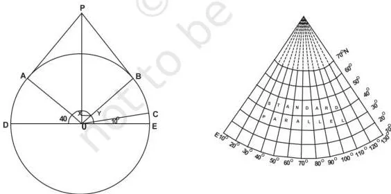
Figure 4.3 shows the finished conical graticule. Note the three details to mention in an answer: the parallels are equally spaced concentric arcs, the meridians are straight lines meeting at the pole, and the pole itself is drawn as an arc (p. 41).
Properties (p. 41)
- All parallels are arcs of concentric circles and are equally spaced.
- All meridians are straight lines meeting at the pole and intersect the parallels at right angles.
- The scale along all meridians is true.
- The pole is represented by an arc of a circle.
- The scale is true along the standard parallel but exaggerated away from it.
- Meridians become closer to each other towards the pole.
- The projection is neither equal-area nor orthomorphic.
Limitations (p. 42)
- Not suitable for a world map because of extreme distortion in the hemisphere opposite the standard parallel.
- Not suitable for very large areas even within the same hemisphere, because distortion grows near the pole and the equator.
Uses (p. 42)
- Areas of mid-latitudes with limited latitudinal but larger longitudinal extent.
- Long narrow strips running parallel to the standard parallel with an east-west stretch.
- Railways, roads, narrow river valleys and international boundaries — for example the Canadian Pacific Railway, the Trans-Siberian Railway, the USA-Canada boundary and the Narmada Valley.
Worked Example 2: Cylindrical Equal Area Projection (Lambert’s)
Lambert’s projection is made by projecting the globe with parallel rays on a cylinder touching it at the equator (NCERT, p. 42). The result is that the pole is shown with a parallel equal to the equator, which is why high-latitude shapes get badly distorted.
Problem. Construct a cylindrical equal area projection for the world at R.F. 1:320,000,000 with a 15° interval.
Step 1 — radius of the reduced earth.
\( R = \frac{640{,}000{,}000}{320{,}000{,}000} = 2.0\ \text{cm} \).
Step 2 — length of the equator.
\( 2\pi R = 2 \times \frac{22}{7} \times 2.0 \approx 12.6\ \text{cm} \).
Step 3 — interval along the equator.
\( \frac{12.6 \times 15^\circ}{360^\circ} = 0.525\ \text{cm} \), which means the 12.6-cm equator is divided into 24 equal parts.
Step 4 — construct the graticule.
- Draw a circle of radius 2.0 cm and mark 15°, 30°, 45°, 60°, 75° and 90° for both hemispheres.
- Draw the equator line 12.6 cm long and divide it into 24 divisions of 0.525 cm.
- Draw a line perpendicular to the equator at the point where 0° meets the circle.
- Extend every parallel so that it is equal in length to the equator.
- Complete the projection as shown in Figure 4.4.
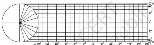
Figure 4.4 shows the finished grid: every parallel and meridian is a straight line and they all intersect at right angles. The polar parallel is as long as the equator — that is why shapes at high latitudes stretch even though areas stay correct.
Properties (p. 43)
- All parallels and meridians are straight lines intersecting at right angles.
- The polar parallel is equal to the equator.
- The scale is true only along the equator.
Limitations (p. 43)
- Distortion increases towards the pole.
- The projection is non-orthomorphic.
- Equality of area is maintained at the cost of distortion in shape.
Uses (p. 43)
- Areas lying between 45°N and 45°S.
- Distribution of tropical crops such as rice, tea, coffee, rubber and sugarcane.
Worked Example 3: Mercator’s Projection
Mercator’s projection was developed by the Dutch cartographer Gerardus Mercator in 1569 and is based on mathematical formulae (NCERT, p. 44). It is orthomorphic: the correct shape is maintained while the distance between parallels increases polewards.
Problem. Draw a Mercator world map at R.F. 1:200,000,000 with a 15° interval.
Step 1 — radius of the reduced earth.
\( R = \frac{640{,}000{,}000}{200{,}000{,}000} = 3.2\ \text{cm} \).
Step 2 — length of the equator.
\( 2\pi R = 2 \times \frac{22}{7} \times 3.2 \approx 20.1\ \text{cm} \).
Step 3 — interval along the equator.
\( \frac{20.1 \times 15^\circ}{360^\circ} \approx 0.84\ \text{cm} \).
Step 4 — latitude distances. Multiply the table values by R = 3.2 cm: 15° → 0.85 cm; 30° → 1.76 cm; 45° → 2.82 cm; 60° → 4.21 cm; 75° → 6.49 cm.
Step 5 — construct the graticule.
- Draw the equator line 20.1 cm long and divide it into 24 equal parts of 0.84 cm.
- Along a central meridian, mark the latitude distances from Step 4 on both sides of the equator.
- Through these marks draw parallels parallel to the equator; through the equator divisions draw meridians.
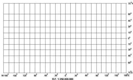
Figure 4.5 is the visual signature of Mercator: parallel spacing widens polewards while meridian spacing stays equal. All parallels are the same length as the equator, and all meridians are equally spaced but longer than the corresponding meridians on the globe (p. 45).
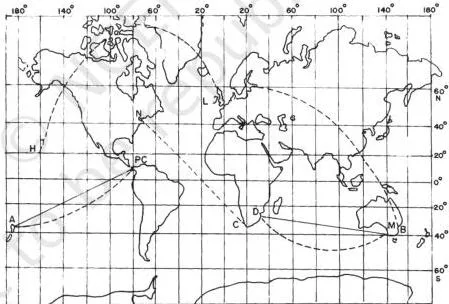
Figure 4.6 contrasts the two navigation lines. A straight line on Mercator gives a constant bearing — the loxodrome or rhumb line, useful in navigation (p. 36, 44). A dotted great circle is the shortest route between two points and is used in air and ocean navigation (p. 36).
Properties (p. 45)
- All parallels and meridians are straight lines intersecting at right angles.
- All parallels are equal in length to the equator.
- All meridians are equal in length and equally spaced, but longer than the corresponding meridians on the globe.
- Spacing between parallels increases towards the pole.
- Scale is correct along the equator; other parallels are longer than the corresponding globe parallel, so the scale is not correct along them. The 30° parallel is 1.154 times longer than on the globe.
- Shape of an area is maintained, but distortion increases at higher latitudes.
- Shape of small countries near the equator is truly preserved.
- It is an azimuthal projection.
- It is an orthomorphic projection because the scale along the meridian equals the scale along the parallel.
Limitations (p. 46)
- Scale is greatly exaggerated along parallels and meridians in high latitudes. Greenland appears equal in size to the USA, though it is only 1/10th of the USA.
- The poles cannot be shown, because the 90° parallel and the meridian touching it are infinite.
Uses (p. 46)
- World maps and atlas maps.
- Navigation — sea routes and air routes.
- Drainage patterns, ocean currents, temperature, winds and their directions, and the distribution of worldwide rainfall and other weather elements.
Two Edge Cases to Remember
- Standard parallel is always the mid parallel of the given range. In Worked Example 1 the latitude list was 20, 30, 40, 50, 60, so the standard parallel is 40°N, not an arbitrary line (p. 40).
- Mercator belongs to two global-property classes. NCERT lists it as both an azimuthal projection and an orthomorphic projection (p. 45) — it preserves direction and shape at the same time, which surprises most students.
Common Mistakes in Map Projections (and the Fix)
| Mistake | Correct rule | How to check your answer |
|---|---|---|
| Mixing up the light sources | Gnomonic = light at the centre; stereographic = light at the periphery diametrically opposite the tangent point; orthographic = light at infinity (p. 40) | Say where the light is before naming the projection. |
| Thinking Mercator preserves area | Mercator is orthomorphic: shapes and directions are correct, but areas inflate polewards (p. 45–46) | Ask “shape or area?” — Mercator keeps shape, not size. |
| Thinking Lambert’s cylindrical equal area keeps correct shapes | It is equal-area: the polar parallel is drawn equal to the equator, so high-latitude shapes distort (p. 43) | Check the polar parallel: equal to the equator means shape is sacrificed. |
| Claiming scale is true across the whole map | No projection keeps scale correct throughout; it is true only along selected lines — the equator for Lambert’s and Mercator, the meridians and standard parallel for conical (pp. 39, 41, 43, 45) | Write down the exact line along which scale is true. |
| Choosing the wrong standard parallel or central meridian | They are the mid values of the given latitude and longitude ranges (p. 40) | Recompute the midpoint of each range. |
| Mixing cm and inch units in Mercator sums | The NCERT Mercator example is worked in inches; this page uses cm, but the formula is identical (p. 44) | Label the unit at every calculated step. |
| Describing conical meridians as curves | Conical meridians are straight lines converging at the pole; the pole itself is an arc (p. 41) | Visualise the cone: its sides are straight, meeting at the apex. |
| Calling the graticule the projection | The graticule is the network of parallels and meridians; the projection is its drawing on a plane (p. 35) | Ask “network or drawing?” — projection is the drawing. |
Misconception autopsy: Mercator is not an equal-area map
The most common confusion is treating the familiar Mercator world map as accurate in area. In fact Mercator is orthomorphic — it preserves shape and direction, but its scale is exaggerated at high latitudes. NCERT gives the standard example: Greenland appears equal to the USA, although it is only 1/10th of the USA (p. 46).
The equal-area compensation works the other way. Lambert’s cylindrical equal area projection keeps area by drawing every parallel, including the pole, equal to the equator — and that is exactly why its shapes stretch at high latitudes (p. 43). In short: Mercator keeps shape, not size; Lambert’s keeps size, not shape.
How to Answer the Chapter’s Exercise Questions
The exercise on pages 47–48 asks for different lengths of answer. This is guidance on answer structure, not a worked answer key.
| Question type | What a complete answer needs |
|---|---|
| Choose-the-right-answer questions (Q1) | Decide which classification base the option belongs to — light source, global property or developable surface — then apply the definition to every option. |
| About-30-word answers (Q2) | Open with a definition sentence, then one supporting point. For (i) name the four elements of projection; for (ii) list the four global properties; for (iii) explain that the globe is non-developable, so distortion is inevitable; for (iv) say that every parallel, including the pole, is extended equal to the equator. |
| Differentiate questions (Q3) | Use point-by-point contrast, not two separate descriptions. Developable vs non-developable = can vs cannot be flattened without breaking or creasing; homolographic vs orthomorphic = equal area vs true shape (do not confuse orthomorphic with the light-source orthographic); normal vs oblique = tangency at the equator vs between pole and equator; parallels vs meridians = unequal circles vs pole-to-pole semi-circles. |
| Not-more-than-125-word answers (Q4) | For classification, name the four bases and the characteristics of each type. For navigation, name Mercator, then state its properties and limitations. For the conical projection, give the main properties and the major limitations. |
| Construction practicals (Activity, p. 48) | Follow the order: calculation → labelled construction steps → properties. Check the standard parallel and central meridian, and keep one unit (cm) throughout. |
Where You Meet These Projections in Real Life
NCERT itself links each projection to a purpose: conical for mid-latitude strips such as railways, roads and boundaries; Lambert’s for tropical crop distributions; Mercator for atlas maps and navigation (pp. 42, 43, 46).
Extension — your phone’s map. Most online maps use a web variant of Mercator’s projection. The chapter does not discuss web maps, but the familiar straight east-west and north-south streets on a phone screen come from the same grid idea as Figure 4.5.
Extension — curved flight paths. Aircraft fly along great circles because they are the shortest routes (p. 36). When that shortest route is drawn on a flat Mercator-style map, it appears as a curve — which is why flight paths arc across oceans.
Extension — why ships steer rhumb lines. A constant bearing is a straight loxodrome or rhumb line on a Mercator chart (pp. 36, 44). A navigator can therefore plot a steady course with a straight edge, instead of constantly changing direction to follow a great circle.
Reading the Chapter’s Diagrams at a Glance
Each figure in the chapter was taught in its section above. Use this table to recall the whole chapter from its diagrams.
| Figure | Page | What it shows | The one detail to remember |
|---|---|---|---|
| 4.1 | 38 | Conversion of a globe to a flat surface | Distortion in area, shape and directions is there from the start. |
| 4.2 | 39 | A conical projection from globe to flat map | A cone is wrapped round the globe, then cut open. |
| 4.3 | 41 | Simple conical projection with one standard parallel | Parallels are concentric arcs; meridians are straight lines meeting at the pole; the pole is an arc. |
| 4.4 | 43 | Cylindrical equal area projection | The polar parallel equals the equator — hence shape loss at high latitudes. |
| 4.5 | 45 | Mercator’s projection | Parallel spacing widens polewards while meridian spacing stays equal. |
| 4.6 | 46 | Rhumb lines and great circles | Straight line = rhumb line; dotted line = great circle. |
You will meet the same graticule ideas again when you read real survey sheets in the topographical maps notes.
Quick Revision: One-Page Recap
| Projection | How the graticule looks | Scale is true along | Preserves | Distorts | Main use |
|---|---|---|---|---|---|
| Conical with one standard parallel | Parallels are equally spaced concentric arcs; meridians are straight lines meeting at the pole and crossing parallels at right angles; pole shown as an arc | All meridians and the standard parallel | Distances along meridians; directions along the standard parallel | Neither equal area nor orthomorphic; distortion grows away from the standard parallel | Mid-latitude strips — railways, roads, river valleys, boundaries |
| Lambert’s cylindrical equal area | Straight lines intersecting at right angles; polar parallel equal to the equator | Only the equator | Area | Shape, increasingly towards the poles | Regions between 45°N and 45°S; tropical crop distribution |
| Mercator | Straight lines at right angles; parallel spacing widens polewards; meridians equally spaced | Only the equator | Shape (orthomorphic) and direction (azimuthal); straight rhumb lines | Area, exaggerated polewards; poles cannot be shown | World and atlas maps, sea and air navigation, weather maps |
The four classification bases in one line each
- Drawing technique: perspective, non-perspective, mathematical/conventional.
- Developable surface: cylindrical, conical, zenithal — subdivided into normal, oblique and polar.
- Global property: equal area, orthomorphic, azimuthal, equidistant.
- Source of light: gnomonic, stereographic, orthographic.
Five one-line takeaways
- The globe is accurate but non-developable, so flattening it must distort something.
- The graticule is the network of parallels and meridians; the projection is its drawing on a plane.
- No projection preserves all four ADDS properties — Area, Direction, Distance, Shape — at once.
- Scale is true only along selected lines, never throughout a map.
- Mercator keeps shape and direction, Lambert’s keeps area, and the conical projection keeps mid-latitude distances.
Try These Constructions Yourself
The chapter ends with an Activity (NCERT, p. 48) containing three graticule constructions. They use exactly the recipes above. Use the radius formula \( R = \frac{640{,}000{,}000}{\text{R.F. denominator}} \) to check the first number of each.
- Simple conical: area between 30°N and 70°N and 40°E and 30°W, scale 1:200,000,000, interval 10°. Checkpoint: \( R = \frac{640{,}000{,}000}{200{,}000{,}000} = 3.2\ \text{cm} \).
- Cylindrical equal area: world at R.F. 1:150,000,000, interval 15°. Checkpoint: \( R = \frac{640{,}000{,}000}{150{,}000{,}000} \approx 4.3\ \text{cm} \).
- Mercator: world at R.F. 1:400,000,000, interval 20°. Checkpoint: \( R = \frac{640{,}000{,}000}{400{,}000{,}000} = 1.6\ \text{cm} \).
Before constructing, verify that the range divides evenly by the interval, choose the mid parallel and mid meridian, and keep every length in cm.
Frequently Asked Questions
Why does every map projection distort something?
Because the globe is a non-developable surface — it cannot be flattened without shrinking, breaking or creasing (NCERT, p. 38). The distortion grows with distance from the tangential point (p. 36), and no projection can preserve distance, shape, area and direction all at once (p. 39). Every projection chooses which property to keep.
Which projection is most useful for navigation and why?
Mercator’s projection is the navigational map. On it, a straight line joining any two points has a constant bearing — a loxodrome or rhumb line — so a navigator can plot a course as a straight line (p. 44). NCERT lists Mercator as useful for sea routes and air routes (p. 46). Its main weakness is area exaggeration at high latitudes.
Why does Greenland look so large on a Mercator map?
Mercator exaggerates scale along the parallels and meridians in high latitudes, so the size of countries near the poles is highly exaggerated. Greenland appears equal in size to the USA, although it is actually only 1/10th of the USA (p. 46).
What is the difference between a rhumb line and a great circle?
A rhumb line joins two points with a constant bearing and is a straight line on Mercator’s projection; it is very useful in navigation (p. 36). A great circle represents the shortest route between two points and is often used in both air and ocean navigation (p. 36).
On a Mercator map, the straight rhumb line and the dotted great-circle arc between the same two points look very different (Fig. 4.6, p. 46).
How do I choose the standard parallel and the central meridian in a conical projection?
Take the mid values of the given ranges. The standard parallel is the middle parallel of the latitude list, and the central meridian is the middle meridian of the longitude list (p. 40). For 10°N to 70°N, for example, the standard parallel is 40°N; for 10°E to 130°E, the central meridian is 70°E.
What is the difference between gnomonic, stereographic and orthographic projections?
The difference is the position of the light source (p. 40). Gnomonic = light at the centre of the globe; stereographic = light at the periphery diametrically opposite the tangent point; orthographic = light at infinity, opposite the tangent point. The G-S-O device — centre, opposite edge, infinity — keeps the order straight.
Reference: NCERT Class 11 Geography textbook, chapter 4 — Map Projections.
Explore Class 11 Geography Notes
- Class 11 Geography Notes
- Class 11 CBSE Notes
- CBSE Notes for Classes 9 to 12
- Next: Topographical Maps
Class 11 Geography on LearnCBSE:
Official source: download the NCERT textbook free from ncert.nic.in.