
This page collects the Motion in a Plane Class 11 formulas from this NCERT chapter: vector addition, subtraction and resolution, kinematic equations for motion in a plane, projectile motion and uniform circular motion. Every formula below carries the meaning of its symbols and their SI units, so you can apply it directly to numericals.
The formulas are grouped by the chapter’s sub-topics, and the quick-reference table after this intro lists every formula on the sheet. You will also find when-to-use guidance, three original worked examples and chapter-specific mistakes to avoid. Formula sheets for the rest of the syllabus are collected in the Class 11 Physics formulas hub.
Formulas at a Glance
The table is the index for this sheet: every formula that appears in the grouped list below, in one place.
| Purpose | Formula |
|---|---|
| Scaling a vector by a real number | \( |\lambda \mathbf{A}| = \lambda |\mathbf{A}| \ (\lambda \gt 0) \) |
| Commutative and associative laws of addition | \( \mathbf{A}+\mathbf{B} = \mathbf{B}+\mathbf{A};\ (\mathbf{A}+\mathbf{B})+\mathbf{C} = \mathbf{A}+(\mathbf{B}+\mathbf{C}) \) |
| Subtracting vectors | \( \mathbf{A}-\mathbf{B} = \mathbf{A}+(-\mathbf{B}) \) |
| Null-vector properties | \( \mathbf{A}+\mathbf{0} = \mathbf{A},\ \lambda\mathbf{0} = \mathbf{0},\ 0\mathbf{A} = \mathbf{0} \) |
| Vector in component form | \( \mathbf{A} = A_x\hat{\mathbf{i}} + A_y\hat{\mathbf{j}} \) |
| Components from magnitude and direction | \( A_x = A\cos\theta,\ A_y = A\sin\theta \) |
| Magnitude from components | \( A = \sqrt{A_x^2+A_y^2} \) |
| Direction from components | \( \tan\theta = \dfrac{A_y}{A_x} \) |
| Three-dimensional vector and its magnitude | \( \mathbf{A} = A_x\hat{\mathbf{i}}+A_y\hat{\mathbf{j}}+A_z\hat{\mathbf{k}},\ A = \sqrt{A_x^2+A_y^2+A_z^2} \) |
| Position vector | \( \mathbf{r} = x\hat{\mathbf{i}}+y\hat{\mathbf{j}}+z\hat{\mathbf{k}} \) |
| Resultant by component addition | \( \mathbf{R} = (A_x+B_x)\hat{\mathbf{i}} + (A_y+B_y)\hat{\mathbf{j}} \) |
| Resultant magnitude of two vectors (law of cosines) | \( R = \sqrt{A^2+B^2+2AB\cos\theta} \) |
| Direction of the resultant | \( \tan\alpha = \dfrac{B\sin\theta}{A+B\cos\theta} \) |
| Displacement vector | \( \Delta\mathbf{r} = \mathbf{r}’-\mathbf{r} = \Delta x\hat{\mathbf{i}}+\Delta y\hat{\mathbf{j}} \) |
| Average velocity | \( \bar{\mathbf{v}} = \dfrac{\Delta\mathbf{r}}{\Delta t} \) |
| Velocity (instantaneous) | \( \mathbf{v} = \dfrac{d\mathbf{r}}{dt} = v_x\hat{\mathbf{i}}+v_y\hat{\mathbf{j}} \) |
| Speed and direction of motion | \( v = \sqrt{v_x^2+v_y^2},\ \tan\theta = \dfrac{v_y}{v_x} \) |
| Average and instantaneous acceleration | \( \bar{\mathbf{a}} = \dfrac{\Delta\mathbf{v}}{\Delta t},\ \mathbf{a} = \dfrac{d\mathbf{v}}{dt} = a_x\hat{\mathbf{i}}+a_y\hat{\mathbf{j}} \) |
| Velocity with constant acceleration | \( \mathbf{v} = \mathbf{v}_0+\mathbf{a}t \) |
| Position with constant acceleration | \( \mathbf{r} = \mathbf{r}_0+\mathbf{v}_0t+\frac{1}{2}\mathbf{a}t^2 \) |
| Constant-acceleration equations in components | \( x = x_0+v_{0x}t+\frac{1}{2}a_xt^2,\ y = y_0+v_{0y}t+\frac{1}{2}a_yt^2 \) |
| Projectile initial-velocity components | \( v_{0x} = v_0\cos\theta_0,\ v_{0y} = v_0\sin\theta_0 \) |
| Projectile position at time t | \( x = (v_0\cos\theta_0)t,\ y = (v_0\sin\theta_0)t-\frac{1}{2}gt^2 \) |
| Projectile velocity at time t | \( v_x = v_0\cos\theta_0,\ v_y = v_0\sin\theta_0-gt \) |
| Equation of the projectile path | \( y = (\tan\theta_0)x-\dfrac{gx^2}{2(v_0\cos\theta_0)^2} \) |
| Time to maximum height | \( t_m = \dfrac{v_0\sin\theta_0}{g} \) |
| Time of flight | \( T_f = \dfrac{2v_0\sin\theta_0}{g} \) |
| Maximum height | \( h_m = \dfrac{(v_0\sin\theta_0)^2}{2g} \) |
| Horizontal range at the same level | \( R = \dfrac{v_0^2\sin 2\theta_0}{g}\ (R_{\max} = \dfrac{v_0^2}{g} \text{ at } \theta_0 = 45^\circ) \) |
| Centripetal acceleration | \( a_c = \dfrac{v^2}{R} \) |
| Angular speed | \( \omega = \dfrac{\Delta\theta}{\Delta t} \) |
| Linear speed from angular speed | \( v = R\omega \) |
| Centripetal acceleration with angular speed | \( a_c = \omega^2R \) |
| Period and frequency relations | \( \omega = \frac{2\pi}{T} = 2\pi\nu,\ v = 2\pi R\nu,\ a_c = 4\pi^2\nu^2R \) |
All Formulas, Grouped by Topic
The grouping follows the NCERT chapter order: start with vector algebra, then kinematics, projectile motion and uniform circular motion.
Multiplication of Vectors by Real Numbers
Multiplying a vector by a positive number \( \lambda \) changes only its magnitude; the direction stays the same (NCERT, Eq. 3.3). A negative multiplier reverses the direction.
\[ |\lambda \mathbf{A}| = \lambda |\mathbf{A}| \quad (\lambda \gt 0) \]
If \( \lambda = 0 \), the product is the null vector \( \mathbf{0} \). If \( \lambda \) is itself a physical quantity, the product carries its dimension: velocity multiplied by time gives displacement.
Addition and Subtraction of Vectors — Graphical Method
Vectors are added by the head-to-tail (triangle) method or, equivalently, the parallelogram method (NCERT, Eqs. 3.1–3.5).
\[ \mathbf{A}+\mathbf{B} = \mathbf{B}+\mathbf{A} \]
\[ (\mathbf{A}+\mathbf{B})+\mathbf{C} = \mathbf{A}+(\mathbf{B}+\mathbf{C}) \]
\[ \mathbf{A}-\mathbf{B} = \mathbf{A}+(-\mathbf{B}) \]
The null vector \( \mathbf{0} \) has zero magnitude, so its direction is not specified. Its properties:
\[ \mathbf{A}+\mathbf{0} = \mathbf{A}, \qquad \lambda\mathbf{0} = \mathbf{0}, \qquad 0\mathbf{A} = \mathbf{0} \]
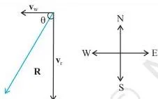
The chapter’s first example uses the triangle method on velocities: rain falling vertically and a horizontal wind produce a resultant R, and the umbrella is held along R (Fig. 3.7). This is exactly the situation where you add two non-parallel vectors to get a resultant.
Resolution of Vectors
Any vector in a plane can be written as a sum of two component vectors. Using unit vectors \( \hat{\mathbf{i}} \) and \( \hat{\mathbf{j}} \) along the x- and y-axes (NCERT, Eqs. 3.12–3.15):
\[ \mathbf{A} = A_x\hat{\mathbf{i}} + A_y\hat{\mathbf{j}} \]
\[ A_x = A\cos\theta, \qquad A_y = A\sin\theta \]
\[ A = \sqrt{A_x^2+A_y^2}, \qquad \tan\theta = \frac{A_y}{A_x} \]
Note that \( \theta \) is measured from the x-axis, so a component can be positive, negative or zero depending on \( \theta \). In three dimensions the same idea uses three perpendicular unit vectors:
\[ \mathbf{A} = A_x\hat{\mathbf{i}} + A_y\hat{\mathbf{j}} + A_z\hat{\mathbf{k}}, \qquad A = \sqrt{A_x^2+A_y^2+A_z^2} \]
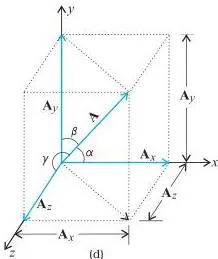
The figure shows how a general vector in space is broken into three perpendicular components, each obtained by projecting the vector on that axis.
Vector Addition — Analytical Method
Component-wise addition is the accurate alternative to drawing. For \( \mathbf{R} = \mathbf{A}+\mathbf{B} \) (NCERT, Eq. 3.21):
\[ R_x = A_x+B_x, \qquad R_y = A_y+B_y \]
For two vectors of magnitudes A and B with angle \( \theta \) between them, the resultant magnitude follows the law of cosines (NCERT, Eq. 3.24a):
\[ R = \sqrt{A^2+B^2+2AB\cos\theta} \]
and its direction is given by (NCERT, Eq. 3.24f):
\[ \tan\alpha = \frac{B\sin\theta}{A+B\cos\theta} \]
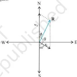
The parallelogram method applied to the boat-and-current example: two velocities drawn from one origin, with the diagonal of the parallelogram as the resultant (Fig. 3.11).
Motion in a Plane: Position, Displacement, Velocity and Acceleration
The position vector \( \mathbf{r} = x\hat{\mathbf{i}}+y\hat{\mathbf{j}} \) describes a particle’s location. Displacement joins the initial and final positions directly and does not depend on the path taken (NCERT, Eq. 3.26):
\[ \Delta\mathbf{r} = \mathbf{r}’-\mathbf{r} = \Delta x\hat{\mathbf{i}} + \Delta y\hat{\mathbf{j}} \]
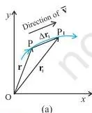
The displacement vector is the straight line between two positions; the path length can be larger, but never smaller.
Velocity is the limiting value of \( \Delta\mathbf{r}/\Delta t \) (NCERT, Eqs. 3.27–3.30c):
\[ \bar{\mathbf{v}} = \frac{\Delta\mathbf{r}}{\Delta t}, \qquad \mathbf{v} = \lim_{\Delta t \to 0}\frac{\Delta\mathbf{r}}{\Delta t} = \frac{d\mathbf{r}}{dt} = v_x\hat{\mathbf{i}}+v_y\hat{\mathbf{j}} \]
\[ v = \sqrt{v_x^2+v_y^2}, \qquad \tan\theta = \frac{v_y}{v_x} \]
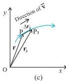
As the time interval shrinks, the average velocity approaches the instantaneous velocity, which is tangent to the path at every point (Fig. 3.13). Acceleration is the corresponding derivative of velocity:
\[ \bar{\mathbf{a}} = \frac{\Delta\mathbf{v}}{\Delta t}, \qquad \mathbf{a} = \lim_{\Delta t \to 0}\frac{\Delta\mathbf{v}}{\Delta t} = \frac{d\mathbf{v}}{dt} = a_x\hat{\mathbf{i}}+a_y\hat{\mathbf{j}} \]
In a plane, the angle between velocity and acceleration can be anywhere from \( 0^\circ \) to \( 180^\circ \), so the two need not point along the same line.
Motion in a Plane with Constant Acceleration
If the acceleration vector is constant, the average acceleration equals it, giving the kinematic equations (NCERT, Eqs. 3.33a–3.34b):
\[ \mathbf{v} = \mathbf{v}_0+\mathbf{a}t \]
\[ \mathbf{r} = \mathbf{r}_0+\mathbf{v}_0t+\frac{1}{2}\mathbf{a}t^2 \]
In component form, with \( v_{0x}, v_{0y} \) the initial velocity components:
\[ v_x = v_{0x}+a_xt, \qquad v_y = v_{0y}+a_yt \]
\[ x = x_0+v_{0x}t+\frac{1}{2}a_xt^2, \qquad y = y_0+v_{0y}t+\frac{1}{2}a_yt^2 \]
This is the chapter’s key result: two-dimensional motion is the superposition of two independent one-dimensional motions along perpendicular directions. Projectile motion is the standard example.
Projectile Motion
For a projectile with air resistance neglected, \( a_x = 0 \) and \( a_y = -g \). The initial velocity components (NCERT, Eq. 3.36):
\[ v_{0x} = v_0\cos\theta_0, \qquad v_{0y} = v_0\sin\theta_0 \]
Position and velocity at time t (NCERT, Eqs. 3.37–3.38):
\[ x = (v_0\cos\theta_0)t, \qquad y = (v_0\sin\theta_0)t-\frac{1}{2}gt^2 \]
\[ v_x = v_0\cos\theta_0, \qquad v_y = v_0\sin\theta_0-gt \]
The horizontal velocity stays constant; the vertical motion is free fall. Eliminating t between x and y gives the path (NCERT, Eq. 3.39):
\[ y = (\tan\theta_0)x-\frac{gx^2}{2(v_0\cos\theta_0)^2} \]
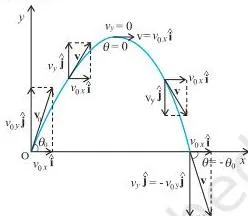
The form \( y = ax+bx^2 \) with constants a and b is a parabola, so the projectile path is parabolic (Fig. 3.17). At maximum height, \( v_y = 0 \); the motion is symmetric about the maximum height, so \( T_f = 2t_m \). The derived results (NCERT, Eqs. 3.40a–3.42b):
\[ t_m = \frac{v_0\sin\theta_0}{g}, \qquad T_f = \frac{2v_0\sin\theta_0}{g} \]
\[ h_m = \frac{(v_0\sin\theta_0)^2}{2g}, \qquad R = \frac{v_0^2\sin 2\theta_0}{g} \]
For a fixed launch speed, R is maximum when \( \sin 2\theta_0 = 1 \), i.e. \( \theta_0 = 45^\circ \), giving \( R_{\max} = v_0^2/g \). This is why the range formula contains \( \sin 2\theta_0 \) rather than \( \sin\theta_0 \).
Uniform Circular Motion
In uniform circular motion the speed is constant but the velocity keeps changing direction, so the acceleration points toward the centre (NCERT, Eq. 3.43):
\[ a_c = \frac{v^2}{R} \]
Angular speed (NCERT, Eq. 3.44) and the link between linear and angular quantities (NCERT, Eq. 3.45):
\[ \omega = \frac{\Delta\theta}{\Delta t}, \qquad v = R\omega \]
Hence (NCERT, Eq. 3.46):
\[ a_c = \omega^2R \]
With time period T and frequency \( \nu \) (NCERT writes italic v for frequency):
\[ \omega = \frac{2\pi}{T} = 2\pi\nu, \qquad v = \frac{2\pi R}{T} = 2\pi R\nu, \qquad a_c = 4\pi^2\nu^2R \]
The magnitude of \( a_c \) is constant, but the vector is not: its direction changes continuously, always pointing to the centre. For this reason the constant-acceleration equations do not apply to uniform circular motion.
What Each Symbol Means
Units follow SI; dimensions are written in the form used in the NCERT summary table. A vector’s unit and dimension are those of the physical quantity it represents.
| Symbol | What it means | SI unit | Dimensions |
|---|---|---|---|
| \( \mathbf{A}, \mathbf{B}, \mathbf{R} \) | Vectors (displacement, velocity, acceleration, force, …) | depends on the quantity (m, m s⁻¹, m s⁻², N) | depends on the quantity |
| \( A = |\mathbf{A}| \) | Magnitude (absolute value) of vector \( \mathbf{A} \) | same as \( \mathbf{A} \) | same as \( \mathbf{A} \) |
| \( \lambda \) | Real number multiplying a vector | dimensionless, or its own physical dimension (e.g. time) | — |
| \( \theta \) | Angle of a vector with the x-axis, or angle between two vectors | degree or radian | dimensionless |
| \( \hat{\mathbf{i}}, \hat{\mathbf{j}}, \hat{\mathbf{k}} \) | Unit vectors along the x-, y- and z-axes | no unit (magnitude 1) | dimensionless |
| \( A_x, A_y \) | Components of \( \mathbf{A} \) along the x- and y-axes | same as \( \mathbf{A} \) | same as \( \mathbf{A} \) |
| \( \mathbf{r} \) | Position vector | m | [L] |
| \( \Delta\mathbf{r} \) | Displacement vector | m | [L] |
| \( \bar{\mathbf{v}} \) | Average velocity \( = \Delta\mathbf{r}/\Delta t \) | m s⁻¹ | [LT⁻¹] |
| \( \mathbf{v} \) | Velocity (instantaneous) \( = d\mathbf{r}/dt \) | m s⁻¹ | [LT⁻¹] |
| \( v_x, v_y \) | Components of velocity | m s⁻¹ | [LT⁻¹] |
| \( \bar{\mathbf{a}} \) | Average acceleration \( = \Delta\mathbf{v}/\Delta t \) | m s⁻² | [LT⁻²] |
| \( \mathbf{a} \) | Acceleration (instantaneous) \( = d\mathbf{v}/dt \) | m s⁻² | [LT⁻²] |
| \( a_x, a_y \) | Components of acceleration | m s⁻² | [LT⁻²] |
| \( \mathbf{v}_0 \) | Initial velocity (velocity at t = 0) | m s⁻¹ | [LT⁻¹] |
| \( v_{0x}, v_{0y} \) | Components of the initial velocity | m s⁻¹ | [LT⁻¹] |
| \( \mathbf{r}_0 \) | Position vector at t = 0 | m | [L] |
| \( t \) | Time elapsed since t = 0 | s | [T] |
| \( g \) | Acceleration due to gravity (≈ 9.8 m s⁻²) | m s⁻² | [LT⁻²] |
| \( \theta_0 \) | Angle of projection with the horizontal | degree or radian | dimensionless |
| \( t_m \) | Time to reach maximum height | s | [T] |
| \( T_f \) | Total time of flight | s | [T] |
| \( h_m \) | Maximum height reached by the projectile | m | [L] |
| \( R \) | Horizontal range | m | [L] |
| \( R_{\max} \) | Maximum range \( = v_0^2/g \), at \( \theta_0 = 45^\circ \) | m | [L] |
| \( a_c \) | Centripetal acceleration in uniform circular motion | m s⁻² | [LT⁻²] |
| \( \omega \) | Angular speed \( = \Delta\theta/\Delta t \) | rad s⁻¹ | [T⁻¹] |
| \( T \) | Time period (time for one revolution) | s | [T] |
| \( \nu \) | Frequency of revolution (written as italic v in NCERT) | s⁻¹ (Hz) | [T⁻¹] |
| \( \Delta\theta \) | Angular displacement in time \( \Delta t \) | radian | dimensionless |
When to Use Each Formula
Reach for a formula only when its condition is satisfied. This table tells you which situation each one belongs to.
| Formula | Use it when… |
|---|---|
| \( R = \sqrt{A^2+B^2+2AB\cos\theta} \) | Two vectors of known magnitudes act at a known angle \( \theta \) and you need the resultant magnitude. If \( \theta = 90^\circ \) it reduces to \( \sqrt{A^2+B^2} \). |
| \( \tan\alpha = \frac{B\sin\theta}{A+B\cos\theta} \) | The same two-vector situation, and you also need the direction of the resultant. The angle \( \alpha \) is measured from vector A. |
| \( A_x = A\cos\theta, \ A_y = A\sin\theta \) | You need the components of a vector — to add several vectors, or to split initial velocity in projectile motion. \( \theta \) must be measured from the chosen x-axis. |
| \( A = \sqrt{A_x^2+A_y^2}, \ \tan\theta = A_y/A_x \) | Components are given and you need the magnitude and direction of the vector. |
| \( \mathbf{v} = d\mathbf{r}/dt, \ \mathbf{a} = d\mathbf{v}/dt \) | Position is given as a function of time. Differentiate once for velocity, twice for acceleration. |
| \( \mathbf{v} = \mathbf{v}_0+\mathbf{a}t, \ \mathbf{r} = \mathbf{r}_0+\mathbf{v}_0t+\frac{1}{2}\mathbf{a}t^2 \) | Acceleration is constant — including projectile motion with \( \mathbf{a} = -g\hat{\mathbf{j}} \). |
| Projectile position equations | The projectile is launched from the origin and you need its position or the time at a given point of the path. Air resistance is neglected. |
| \( h_m = \frac{(v_0\sin\theta_0)^2}{2g}, \ t_m = \frac{v_0\sin\theta_0}{g} \) | Any projectile: at maximum height \( v_y = 0 \), so these two formulas do not depend on where the projectile lands. |
| \( T_f, \ R \) | Only when the projectile lands at the same height it was launched from (y = 0 at both ends). For a cliff or elevated launch, solve the y-equation for t first. |
| \( R_{\max} = v_0^2/g \) | The maximum possible range for a given launch speed, reached at \( \theta_0 = 45^\circ \). |
| \( a_c = v^2/R = \omega^2R \) | Uniform circular motion (speed constant). The acceleration is centripetal — toward the centre. |
| \( v = R\omega, \ \omega = 2\pi/T = 2\pi\nu \) | Converting between linear and angular quantities. Convert revolutions per second to rad s⁻¹ by multiplying by \( 2\pi \). |
Worked Examples
These three examples use original numbers. Each shows the formula being selected, the substitution, and a self-check.
Worked Example 1: Resultant of two vectors by the law of cosines
Step 1: Two displacements act at one point: \( \mathbf{A} = 12\ \text{m} \) east and \( \mathbf{B} = 5\ \text{m} \) at \( 60^\circ \) north of east.
The angle between them is \( \theta = 60^\circ \), so the law of cosines applies (the vectors are not perpendicular).
\[ R = \sqrt{A^2+B^2+2AB\cos\theta} = \sqrt{12^2+5^2+2(12)(5)\cos 60^\circ} \]
\[ R = \sqrt{144+25+120(0.5)} = \sqrt{229} \approx 15.1\ \text{m} \]
Step 2: Direction of \( \mathbf{R} \) measured from \( \mathbf{A} \), using the direction formula:
\[ \tan\alpha = \frac{B\sin\theta}{A+B\cos\theta} = \frac{5\sin 60^\circ}{12+5\cos 60^\circ} = \frac{4.33}{14.5} = 0.299 \Rightarrow \alpha \approx 16.6^\circ \]
Check: Add components — \( R_x = 12+5\cos 60^\circ = 14.5\ \text{m} \), \( R_y = 5\sin 60^\circ = 4.33\ \text{m} \).
Then \( R = \sqrt{14.5^2+4.33^2} = \sqrt{229} \approx 15.1\ \text{m} \), the same result.
Final answer: resultant \( \approx 15.1\ \text{m} \) at \( 16.6^\circ \) north of east.
Worked Example 2: Maximum height, time of flight and range of a projectile
Step 1: A ball is projected at \( v_0 = 50\ \text{m s}^{-1} \) at \( \theta_0 = 37^\circ \) to the horizontal.
Take \( g = 9.8\ \text{m s}^{-2} \).
Resolve the initial velocity: \( v_{0x} = v_0\cos\theta_0 \), \( v_{0y} = v_0\sin\theta_0 \) with \( \sin 37^\circ \approx 0.6018 \).
\[ h_m = \frac{(v_0\sin\theta_0)^2}{2g} = \frac{(50 \times 0.6018)^2}{2 \times 9.8} = \frac{(30.1)^2}{19.6} \approx 46.2\ \text{m} \]
\[ T_f = \frac{2v_0\sin\theta_0}{g} = \frac{2(50)(0.6018)}{9.8} \approx 6.14\ \text{s} \]
\[ R = \frac{v_0^2\sin 2\theta_0}{g} = \frac{2500\sin 74^\circ}{9.8} \approx 245\ \text{m} \]
Check: The midpoint time is \( t_m = T_f/2 = 3.07\ \text{s} \).
Putting it in \( y = v_{0y}t-\frac{1}{2}gt^2 \) gives \( y = 30.1(3.07)-4.9(3.07)^2 \approx 46.2\ \text{m} \), equal to \( h_m \), as it must be.
Final answer: \( h_m \approx 46\ \text{m} \), \( T_f \approx 6.1\ \text{s} \), \( R \approx 245\ \text{m} \).
Worked Example 3: Uniform circular motion — angular speed and centripetal acceleration
Step 1: A particle moves in a circle of radius \( R = 0.80\ \text{m} \) at a constant speed \( v = 6.0\ \text{m s}^{-1} \).
Find the angular speed from \( v = R\omega \):
\[ \omega = \frac{v}{R} = \frac{6.0}{0.80} = 7.5\ \text{rad s}^{-1} \]
Step 2: Centripetal acceleration in two equivalent forms:
\[ a_c = \frac{v^2}{R} = \frac{6.0^2}{0.80} = 45\ \text{m s}^{-2}, \qquad a_c = \omega^2R = (7.5)^2(0.80) = 45\ \text{m s}^{-2} \]
Direction: \( a_c \) points toward the centre at every instant.
Its direction changes as the particle moves, so \( \mathbf{a}_c \) is not a constant vector even though its magnitude is.
Final answer: \( \omega = 7.5\ \text{rad s}^{-1} \), \( a_c = 45\ \text{m s}^{-2} \) directed toward the centre.
Common Mistakes to Avoid
These are the errors students make while applying this chapter’s formulas. Each row includes a quick self-check.
| Mistake | Correct rule | How to check your answer |
|---|---|---|
| Adding two non-perpendicular vectors with \( \sqrt{A^2+B^2} \) | Use \( R = \sqrt{A^2+B^2+2AB\cos\theta} \) whenever the angle between the vectors is not \( 90^\circ \). | Add the components: \( R = \sqrt{R_x^2+R_y^2} \) must give the same value. |
| Writing the direction as \( \tan\theta = A_x/A_y \) | For a vector making angle \( \theta \) with the x-axis, \( \tan\theta = A_y/A_x \). | A vector along +y has components \( (0, A) \); only \( A_y/A_x \) is infinite, giving \( \theta = 90^\circ \). |
| Using \( R = v_0^2\sin 2\theta_0/g \) when the projectile lands at a different height | The range formula is valid only when launch and landing are at the same level (y = 0 at both ends). | For a cliff launch, find t from \( y = v_{0y}t-\frac{1}{2}gt^2 \) and compare \( x = v_{0x}t \) with the range formula — they will differ. |
| Writing \( R = v_0^2/g \) for every projection angle | \( R = v_0^2\sin 2\theta_0/g \). The simpler form \( v_0^2/g \) is only the maximum, at \( \theta_0 = 45^\circ \). | \( \sin 2\theta_0 \leq 1 \) always, so any computed range greater than \( v_0^2/g \) is impossible. |
| Treating centripetal acceleration as a constant vector | Magnitude \( a_c = v^2/R \) is constant, but the direction is always toward the centre and keeps changing, so \( \mathbf{a}_c \) is not constant. | Draw \( \mathbf{a}_c \) at two different points of the circle; both arrows must point to the centre. If they are parallel, you have treated it as constant. |
| Using revolutions per second directly as angular speed | \( \omega = 2\pi/T = 2\pi\nu \) in rad s⁻¹. Frequency must be multiplied by \( 2\pi \) before it becomes \( \omega \). | For \( T = 0.50\ \text{s} \), \( \omega = 2\pi/0.50 \approx 12.6\ \text{rad s}^{-1} \). If you get 2.0, you dropped the \( 2\pi \). |
Frequently Asked Questions
Why is the path of a projectile a parabola?
Eliminating time between \( x = (v_0\cos\theta_0)t \) and \( y = (v_0\sin\theta_0)t-\frac{1}{2}gt^2 \) gives \( y = (\tan\theta_0)x-\frac{gx^2}{2(v_0\cos\theta_0)^2} \), which has the form \( y = ax+bx^2 \). Since \( g \), \( v_0 \) and \( \theta_0 \) are constants during the flight, this is a parabola (NCERT, Eq. 3.39).
At what angle is the horizontal range maximum, and why?
\( R = v_0^2\sin 2\theta_0/g \). For a fixed \( v_0 \), the range is largest when \( \sin 2\theta_0 = 1 \), so \( 2\theta_0 = 90^\circ \) and \( \theta_0 = 45^\circ \), giving \( R_{\max} = v_0^2/g \). Angles that exceed or fall short of \( 45^\circ \) by the same amount give equal ranges, because \( \sin(90^\circ \pm 2\alpha) = \cos 2\alpha \).
Is the acceleration in uniform circular motion constant?
No. The magnitude is constant, \( a_c = v^2/R = \omega^2R \), but the direction is always toward the centre and keeps changing as the object moves. So the acceleration is not a constant vector, and the constant-acceleration equations \( \mathbf{v} = \mathbf{v}_0+\mathbf{a}t \) do not apply to uniform circular motion.
When can I use the formula \( R = v_0^2\sin 2\theta_0/g \)?
Only when the projectile is launched and lands at the same level, so y = 0 at both instants. If it lands at a different height, find the flight time from \( y = (v_0\sin\theta_0)t-\frac{1}{2}gt^2 \) with the actual final value of y, then use \( x = (v_0\cos\theta_0)t \).
Reference: NCERT Class 11 Physics textbook, chapter Motion in a Plane. All formulas follow the Rationalised NCERT text; verify them against the official NCERT website, and find formula sheets for other chapters and classes at the formulas index.
Explore Class 11 Physics Formulas
More for this chapter:
Class 11 Physics on LearnCBSE:
Related chapters: