
These motion in a plane class 11 notes condense NCERT Physics Part I Chapter 3 into a revision-ready guide. The chapter moves beyond the straight line of Chapter 2: in a plane an object can travel in infinitely many directions, so the plus and minus signs that carried direction in one dimension are no longer enough — vectors take over (NCERT, p. 28).
Inside you get the vector rules that reappear in every later physics chapter — addition, resolution, components and the resultant formula — then velocity and acceleration as vectors, projectile motion, and uniform circular motion. Each concept is followed by a definitions table, a formula box with SI units, five original worked examples and a chapter-specific mistakes table.
This page is one of a full set of chapter resources that live on the study notes home.
How to use it: read each concept section once, then attempt the five worked examples before checking the steps — that attempt is what fixes the formulas in your head. Bookmark the formula box near the end for the night before the exam.
Motion in a Plane Class 11 Notes: The Big Picture
In one dimension only two directions exist, so + and − signs describe direction completely. In a plane an object can move in an infinite number of directions, so position, displacement, velocity and acceleration must all be described with vectors (NCERT, p. 28).
One idea unlocks the whole chapter: a two-dimensional motion is two simultaneous one-dimensional motions along perpendicular directions, and these two motions are independent of each other (NCERT, p. 38). Once you accept this, every projectile problem becomes a pair of straight-line problems you already know how to solve.

The build order a teacher follows — and these notes follow — is: scalar/vector language, vector algebra, resolution into components, analytical addition, kinematics as vectors, projectile motion, then uniform circular motion. If the one-dimensional groundwork feels shaky, revise the Motion in a Straight Line notes first, because the projectile analysis assumes them.
| Feature | One-dimensional motion | Two-dimensional motion |
|---|---|---|
| Direction carried by | + and − signs | vectors (components, or magnitude + angle) |
| Position | \( x(t) \) along the line | \( \mathbf{r} = x\hat{\mathbf{i}} + y\hat{\mathbf{j}} \) |
| Displacement | \( \Delta x = x’ – x \) | \( \Delta \mathbf{r} = (\Delta x)\hat{\mathbf{i}} + (\Delta y)\hat{\mathbf{j}} \) |
| Velocity | \( v = dx/dt \) | \( \mathbf{v} = v_x\hat{\mathbf{i}} + v_y\hat{\mathbf{j}} \) |
| Acceleration | \( a = dv/dt \) | \( \mathbf{a} = a_x\hat{\mathbf{i}} + a_y\hat{\mathbf{j}} \) |
| Valid equations | \( v = v_0 + at \), \( x = x_0 + v_0t + \frac{1}{2}at^2 \) | the same equations applied independently along x and y |
| Example path | straight line | parabola, circle |
Scalars vs Vectors: The Two-Rule Test
A scalar quantity has magnitude only — a single number with its unit settles it. A vector quantity has both magnitude and direction, and it must obey the triangle law of addition or, equivalently, the parallelogram law (NCERT, p. 28). That last clause matters: a vector is not just “a quantity with direction” — it must also add the vector way.
Apply the two-rule test to any quantity in an exam list:
- Rule 1 — Does the quantity have a direction? If no, it is a scalar.
- Rule 2 — Does it combine by the triangle/parallelogram (vector) law? If both answers are yes, it is a vector.
In print a vector is shown in bold, \( \mathbf{v} \); written by hand it carries an arrow, \( \vec{v} \). The magnitude is written \( |\mathbf{v}| = v \) (NCERT, p. 28). The standard pair is speed versus velocity — speed is the magnitude of the velocity vector.
| Feature | Scalar | Vector |
|---|---|---|
| Defined by | magnitude only | magnitude + direction |
| Combining rule | ordinary algebra | triangle law = parallelogram law |
| Rule 1: has a direction? | no | yes |
| Rule 2: adds by the vector law? | no | yes |
| Examples | speed, distance, mass, temperature | velocity, displacement, acceleration, force |
This two-rule test is exactly what exercise 3.1 on NCERT p. 47 asks you to apply. Classify this list yourself before moving on: volume, mass, speed, acceleration, density, number of moles, velocity, angular frequency, displacement, angular velocity. (Work through it on your own — the answers are for you to find, not for this page to give away.)
Position and Displacement Vectors
To fix an object’s position in a plane you need an origin. The position vector \( \mathbf{r} \) joins the origin O to the object’s point P, written \( \mathbf{r} = x\hat{\mathbf{i}} + y\hat{\mathbf{j}} \), where x and y are the coordinates of P (NCERT, p. 29).
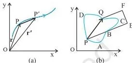
When the object moves from P to P′, the displacement vector is \( \Delta \mathbf{r} = \mathbf{r}’ – \mathbf{r} \), the straight line from the initial point P to the final point P′. In Fig 3.1(b), the displacement is the same straight line PQ whether the object follows path PABCQ, PDQ or PBEFQ.
Displacement depends only on the end points; path length depends on the actual route.
The consequence is an inequality to quote in exams: path length \( \ge |\Delta \mathbf{r}| \), with equality only when the direction of motion never changes (Points to Ponder 1, NCERT, p. 46). In component form, \[ \Delta \mathbf{r} = (x’ – x)\hat{\mathbf{i}} + (y’ – y)\hat{\mathbf{j}} = (\Delta x)\hat{\mathbf{i}} + (\Delta y)\hat{\mathbf{j}} \]
Vector Algebra: Equality, Multiplication and the Null Vector
Two vectors \( \mathbf{A} \) and \( \mathbf{B} \) are equal only if they have the same magnitude and the same direction. Vectors in this chapter are free vectors — shifting a vector parallel to itself leaves it unchanged — so equality is checked by sliding one vector until its tail meets the other’s tail (footnote, NCERT, p. 29).
Fig 3.2(b) is the counter-example: same length, different direction, so the vectors are unequal.
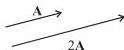
Multiplying a vector by a real number \( \lambda \) scales it: \( |\lambda \mathbf{A}| = \lambda |\mathbf{A}| \) for \( \lambda \gt 0 \), with the direction unchanged. A negative \( \lambda \) reverses the direction; \( \lambda = 0 \) gives the null vector (NCERT, p. 30).
The null vector \( \mathbf{0} \) has zero magnitude, so its direction cannot be specified. It obeys \( \mathbf{A} + \mathbf{0} = \mathbf{A} \), \( \lambda \mathbf{0} = \mathbf{0} \) and \( 0\mathbf{A} = \mathbf{0} \) (Eq. 3.4). A real null displacement appears when an object goes from P to P′ and back to P: initial and final positions coincide, so the displacement is a null vector (NCERT, p. 31).
A subtle physical point: \( \lambda \) may carry a dimension. Multiply a constant velocity vector by a duration of time and you get a displacement vector (NCERT, p. 30) — \( \lambda \mathbf{A} \) need not have the same units as \( \mathbf{A} \).
Adding and Subtracting Vectors Graphically
Triangle (head-to-tail) method: place the tail of \( \mathbf{B} \) at the head of \( \mathbf{A} \); the resultant \( \mathbf{R} = \mathbf{A} + \mathbf{B} \) is the vector from the tail of \( \mathbf{A} \) to the head of \( \mathbf{B} \). Adding in the other order, \( \mathbf{B} + \mathbf{A} \), gives the same \( \mathbf{R} \), so vector addition is commutative (Eq. 3.1).
It is also associative (Eq. 3.2):
\[ \mathbf{A} + \mathbf{B} = \mathbf{B} + \mathbf{A}, \qquad (\mathbf{A} + \mathbf{B}) + \mathbf{C} = \mathbf{A} + (\mathbf{B} + \mathbf{C}) \]
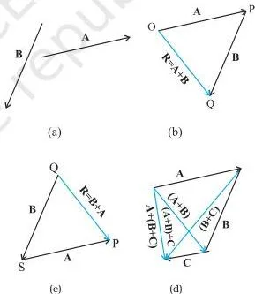
Parallelogram method: bring both tails to a common origin, complete the parallelogram, and the diagonal from the common origin is \( \mathbf{R} \). Fig 3.6(c) shows that the triangle method and the parallelogram method yield the same resultant, so the two are equivalent (NCERT, p. 31).
Both work because a vector is fixed by magnitude and direction alone — the drawing arrangement changes nothing.
Subtraction is addition of the negative: \( \mathbf{A} – \mathbf{B} = \mathbf{A} + (-\mathbf{B}) \) (Eq. 3.5), where \( -\mathbf{B} \) has the same length as \( \mathbf{B} \) but opposite direction.
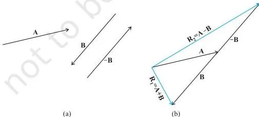
The same rule handles velocity sums — Example 3.1’s rain-and-wind problem is the classic case: the boy’s umbrella must point along the resultant of the rain velocity and the wind velocity. The textbook supplies the numbers; the two-vector addition rule is what you revise.
Resolution of Vectors: Components and Unit Vectors
Any plane vector \( \mathbf{A} \) can be written as a sum of two component vectors: \( \mathbf{A} = \lambda\mathbf{a} + \mu\mathbf{b} \), where \( \mathbf{a} \) and \( \mathbf{b} \) are any two non-collinear vectors in the plane (Eq. 3.8). This is resolution of a vector.
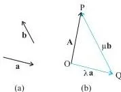
The convenient special case uses rectangular axes and unit vectors. A unit vector has magnitude 1, points in a particular direction, and has no dimension and no unit; \( \hat{\mathbf{i}}, \hat{\mathbf{j}}, \hat{\mathbf{k}} \) lie along the x-, y- and z-axes, perpendicular to each other (NCERT, p. 32).
For \( \mathbf{A} \) in the x-y plane making angle \( \theta \) with the x-axis, \( \mathbf{A} = A_x\hat{\mathbf{i}} + A_y\hat{\mathbf{j}} \), with \[ A_x = A\cos\theta, \qquad A_y = A\sin\theta \qquad (3.13) \]
\[ A = \sqrt{A_x^2 + A_y^2}, \qquad \tan\theta = \frac{A_y}{A_x} \qquad (3.14, 3.15) \]
Two traps hide here. First, \( A_x \) itself is not a vector — it is a number; the vector is \( A_x\hat{\mathbf{i}} \) (NCERT, p. 33). Second, components can be positive, negative or zero depending on where the angle places the vector; the formulas do not force them positive.
| Way to specify a vector | What you provide | Best when |
|---|---|---|
| Magnitude + direction | \( A \) and the angle \( \theta \) with the x-axis | describing motion, drawing diagrams |
| Component form | \( A_x \) and \( A_y \) | adding vectors analytically, computing resultants |
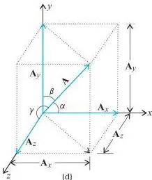
The same procedure extends to three dimensions: \( \mathbf{A} = A_x\hat{\mathbf{i}} + A_y\hat{\mathbf{j}} + A_z\hat{\mathbf{k}} \) with \( A = \sqrt{A_x^2 + A_y^2 + A_z^2} \) (Eqs. 3.16), and the position vector is \( \mathbf{r} = x\hat{\mathbf{i}} + y\hat{\mathbf{j}} + z\hat{\mathbf{k}} \) (Eq. 3.17) — the picture in Fig 3.9(d).
Analytical Addition: The Law of Cosines
Graphical addition is good for pictures but slow for numbers. The analytical method adds component by component: if \( \mathbf{R} = \mathbf{A} + \mathbf{B} \), then \[ R_x = A_x + B_x, \qquad R_y = A_y + B_y \qquad (3.21) \]
Every numerical should start here. When only the magnitudes \( A, B \) and the angle \( \theta \) between them are known, the resultant magnitude comes from the law of cosines, derived from Fig 3.10: drop a perpendicular SN from the head of \( \mathbf{B} \) onto the line of \( \mathbf{A} \) extended. From the geometry of the right triangle OSN:
\[ ON = A + B\cos\theta, \qquad SN = B\sin\theta \]
\[ OS^2 = ON^2 + SN^2 = (A + B\cos\theta)^2 + (B\sin\theta)^2 \]
\[ R = \sqrt{A^2 + B^2 + 2AB\cos\theta} \qquad (3.24a) \]
Its direction, measured from \( \mathbf{A} \), is \[ \tan\alpha = \frac{SN}{ON} = \frac{B\sin\theta}{A + B\cos\theta} \qquad (3.24f) \]
The companion relation, the law of sines, is \( R/\sin\theta = A/\sin\beta = B/\sin\alpha \) (Eq. 3.24d). Why does the derivation work?
The perpendicular SN performs the resolution trick of the previous section — it splits \( \mathbf{B} \) into a part \( B\cos\theta \) along \( \mathbf{A} \) and a part \( B\sin\theta \) perpendicular to it; Pythagoras then combines them.
In exam answers, the step that earns the mark is writing \( ON = A + B\cos\theta \) and \( SN = B\sin\theta \) before applying Pythagoras, so do not skip to the final formula.
Velocity and Acceleration as Vectors
For a particle at \( \mathbf{r} = x\hat{\mathbf{i}} + y\hat{\mathbf{j}} \), the average velocity is \( \bar{\mathbf{v}} = \Delta\mathbf{r}/\Delta t \) and the instantaneous velocity is \( \mathbf{v} = d\mathbf{r}/dt \) (Eqs. 3.27–3.28).
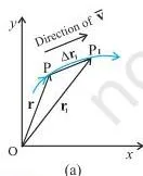
Fig 3.13 is the geometric heart of the limiting process. As the time interval shrinks (\( \Delta t_1 \gt \Delta t_2 \gt \Delta t_3 \)), the displacement \( \Delta\mathbf{r} \) swings around until, in the limit, it lies along the tangent at P. So the velocity at any point is tangential to the path and points in the direction of motion (NCERT, p. 36).
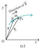
In components: \( v_x = dx/dt \), \( v_y = dy/dt \), with \( v = \sqrt{v_x^2 + v_y^2} \) and \( \tan\theta = v_y/v_x \) (Eqs. 3.30).
Acceleration is defined the same way: average \( \bar{\mathbf{a}} = \Delta\mathbf{v}/\Delta t \), instantaneous \( \mathbf{a} = d\mathbf{v}/dt \), with components \( a_x = dv_x/dt \) and \( a_y = dv_y/dt \) (Eqs. 3.31–3.32).
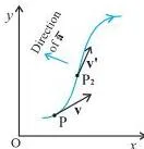
Fig 3.15 shows how \( \Delta\mathbf{v} \), and hence the average acceleration, is constructed by the triangle law for shrinking time intervals. One contrast separates this chapter from the last: in one dimension, velocity and acceleration are always collinear, but in a plane the angle between them can be anything from \( 0^\circ \) to \( 180^\circ \) (NCERT, p. 37).
Given \( \mathbf{r}(t) \), differentiate once for \( \mathbf{v}(t) \) and twice for \( \mathbf{a}(t) \) — the method of Example 3.4. An original numerical of this type appears in the Worked Examples section.
Constant Acceleration: The Two Master Equations
Constant acceleration means the average acceleration over any interval equals the instantaneous value, so the straight-line equations carry over unchanged as vectors:
\[ \mathbf{v} = \mathbf{v}_0 + \mathbf{a}t \qquad (3.33a) \]
\[ \mathbf{r} = \mathbf{r}_0 + \mathbf{v}_0t + \frac{1}{2}\mathbf{a}t^2 \qquad (3.34a) \]
Why the second equation? Displacement equals average velocity times time, and with constant acceleration the average velocity is \( (\mathbf{v}_0 + \mathbf{v})/2 \) — the same argument used for straight-line motion (NCERT, p. 38). In components:
- \( v_x = v_{0x} + a_x t \), \( v_y = v_{0y} + a_y t \)
- \( x = x_0 + v_{0x}t + \frac{1}{2}a_x t^2 \), \( y = y_0 + v_{0y}t + \frac{1}{2}a_y t^2 \)
These pairs expose the chapter’s central result: the x-motion and y-motion are independent of each other. A motion in a plane is two simultaneous one-dimensional motions along perpendicular directions (NCERT, p. 38) — the entire projectile analysis below rests on this idea.
One honest catch from Points to Ponder 4 (NCERT, p. 46): these equations require a constant acceleration vector, so they do not apply to uniform circular motion, where the acceleration keeps changing direction.
Projectile Motion: Parabolic Path, Height, Time and Range
A projectile is any object in flight after being thrown or projected — a football, a cricket ball, a stone. Galileo was the first to state that the horizontal and vertical components of projectile motion act independently (NCERT, p. 39).
Set up with the launch point as origin and acceleration \( \mathbf{a} = -g\hat{\mathbf{j}} \), so \( a_x = 0 \) and \( a_y = -g \). The launch speed \( v_0 \) at angle \( \theta_0 \) above the horizontal splits into \[ v_{0x} = v_0\cos\theta_0, \qquad v_{0y} = v_0\sin\theta_0 \qquad (3.36) \]
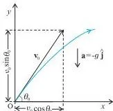
From the master equations come the position and velocity at time \( t \):
\[ x = v_0\cos\theta_0\, t, \qquad y = v_0\sin\theta_0\, t – \frac{1}{2}gt^2 \qquad (3.37) \]
\[ v_x = v_0\cos\theta_0 \ (\text{constant!}), \qquad v_y = v_0\sin\theta_0 – gt \qquad (3.38) \]
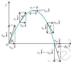
The horizontal component of velocity never changes during the flight; only the vertical component behaves like free fall. Eliminating \( t \) between the x- and y-equations gives the path:
\[ y = (\tan\theta_0)x – \frac{gx^2}{2v_0^2\cos^2\theta_0} \qquad (3.39) \]
which has the form \( y = ax + bx^2 \) — the equation of a parabola (NCERT, p. 39).
| Result | Formula | Where it comes from |
|---|---|---|
| Time of maximum height | \( t_m = \dfrac{v_0\sin\theta_0}{g} \) | set \( v_y = 0 \) in Eq. 3.38 |
| Time of flight | \( T_f = \dfrac{2v_0\sin\theta_0}{g} \) | set \( y = 0 \) in Eq. 3.37; symmetry gives \( T_f = 2t_m \) |
| Maximum height | \( h_m = \dfrac{(v_0\sin\theta_0)^2}{2g} \) | put \( t = t_m \) into the y-equation |
| Horizontal range | \( R = \dfrac{v_0^2\sin 2\theta_0}{g} \) | \( R = v_{0x} \times T_f \) |
| Maximum range | \( R_{\max} = \dfrac{v_0^2}{g} \) at \( \theta_0 = 45^\circ \) | \( \sin 2\theta_0 \) peaks at 1 |
Misconception Autopsy: Is the Projectile at Rest at the Top?
Students write “the projectile stops at maximum height”. The correct picture: only the vertical component vanishes there — \( v_y = 0 \). The horizontal component \( v_x = v_0\cos\theta_0 \) keeps pushing forward, so at the top the projectile is moving horizontally with speed \( v_0\cos\theta_0 \), and the velocity angle there is \( 0^\circ \) (NCERT, p. 39).
The projectile is never at rest; “instantaneously at rest” would need both components to be zero at once.
Memory Device: The Double-Angle Dose
Range wears a double-angle dose: \( 2\theta_0 \) sits inside the sine, and the dose peaks at \( 45^\circ \). One pass — “\( R = v_0^2\sin 2\theta_0/g \), maximum when \( \sin 2\theta_0 = 1 \) at \( 45^\circ \) ” — memorises the formula and its maximum condition together.
Real-Life Application: The Flat Throw vs the Lob
Galileo’s complementary-angle rule (Example 3.6) says angles \( \theta_0 \) and \( 90^\circ – \theta_0 \) give equal ranges, because \( \sin 2(90^\circ – \theta_0) = \sin(180^\circ – 2\theta_0) = \sin 2\theta_0 \). A fielder can therefore reach the same spot with a low flat throw or a high lob — the lob simply stays in the air much longer, which is why high catches feel so slow.
This holds for ideal conditions with no air resistance (NCERT, p. 40).
Uniform Circular Motion: Centripetal Acceleration
Uniform circular motion means a circular path at constant speed. The word “uniform” refers to speed alone; the direction of the velocity changes continuously, so the motion is accelerated (NCERT, p. 41).
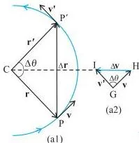
In Fig 3.18 the velocity is tangent at every point.
Bring \( \mathbf{v} \) and \( \mathbf{v}’ \) tail-to-tail: the triangle formed by the position vectors \( (\mathbf{r}, \mathbf{r}’, \Delta\mathbf{r}) \) is similar to the triangle formed by the velocity vectors \( (\mathbf{v}, \mathbf{v}’, \Delta\mathbf{v}) \), because \( \mathbf{v} \) is perpendicular to \( \mathbf{r} \) and \( \mathbf{v}’ \) to \( \mathbf{r}’ \).
Similarity gives \( |\Delta\mathbf{v}|/v = |\Delta\mathbf{r}|/R \). Divide by \( \Delta t \) and take the limit:
\[ |\mathbf{a}| = \lim_{\Delta t \to 0}\frac{|\Delta\mathbf{v}|}{\Delta t} = \frac{v}{R}\lim_{\Delta t \to 0}\frac{|\Delta\mathbf{r}|}{\Delta t} = \frac{v}{R} \times v = \frac{v^2}{R} \qquad (3.43) \]
As \( \Delta t \to 0 \), the direction of \( \Delta\mathbf{v} \) — and hence of the acceleration — points straight at the centre. This is the centripetal (centre-seeking) acceleration, a term proposed by Newton; its full analysis was published by Huygens in 1673 (NCERT, p. 42).
Its magnitude \( v^2/R \) is constant, but its direction changes continuously, so the centripetal acceleration is not a constant vector.
The angular description is shorter: angular speed \( \omega = \Delta\theta/\Delta t \) (Eq. 3.44); since arc length \( \Delta s = R\Delta\theta \), \[ v = R\omega, \qquad a_c = \omega^2R \qquad (3.45, 3.46) \]
With period \( T \) (time for one revolution) and frequency \( \nu = 1/T \) (revolutions per second): \( \omega = 2\pi\nu \), \( v = 2\pi R\nu \), \( a_c = 4\pi^2\nu^2R \) (Eqs. 3.47–3.48).
- The equations \( \mathbf{v} = \mathbf{v}_0 + \mathbf{a}t \) do not apply here, because the acceleration direction keeps changing (Points to Ponder 4, NCERT, p. 46).
- The resultant acceleration points towards the centre only if the speed is constant (Points to Ponder 6, NCERT, p. 46).
- \( a_c \) has constant magnitude but is not a constant vector (NCERT, p. 42).
The forces that produce this acceleration — friction on a turning car, tension in a string, banking of roads — are the subject of the Laws of Motion notes that follow this chapter.
Definitions You Must Know: From Scalar to Centripetal Acceleration
Every examinable term of the chapter, in one table.
| Term | Meaning | Example |
|---|---|---|
| Scalar | quantity with magnitude only, fixed by a number + unit, combined by ordinary algebra | mass of 5 kg |
| Vector | quantity with magnitude and direction that obeys the triangle/parallelogram law | force of 6 N eastward |
| Position vector | vector from the origin to the object’s position | \( \mathbf{r} = x\hat{\mathbf{i}} + y\hat{\mathbf{j}} \) at point P |
| Displacement vector | straight line from initial to final position; independent of the path | a train’s straight-line shift from Delhi to Agra, whatever route it takes |
| Unit vector | vector of magnitude 1, no dimension and no unit, used to specify direction | \( \hat{\mathbf{i}} \) along the x-axis |
| Null (zero) vector | vector of zero magnitude; its direction cannot be specified | displacement of an object that returns to its start |
| Resultant | single vector equal to the sum of given vectors | the diagonal OS of a vector parallelogram |
| Component of a vector | part of a vector along a chosen direction; \( A_x \) is a number, \( A_x\hat{\mathbf{i}} \) is a vector | \( A_x = A\cos\theta \) along x |
| Projectile | object in flight after being thrown or projected | a cricket ball in the air after a throw |
| Time of flight | total time a projectile stays in flight | \( T_f = 2v_0\sin\theta_0/g \) |
| Maximum height | greatest vertical height reached by a projectile | \( h_m = (v_0\sin\theta_0)^2/2g \) |
| Horizontal range | horizontal distance from launch to the point where the projectile returns to the same level | \( R = v_0^2\sin 2\theta_0/g \) |
| Angular speed | rate of change of angular displacement | \( \omega = \Delta\theta/\Delta t \) in rad/s |
| Time period | time for one complete revolution | \( T = 2\pi/\omega \) |
| Frequency | number of revolutions per second | \( \nu = 1/T \) in Hz |
| Centripetal acceleration | acceleration of uniform circular motion, magnitude \( v^2/R \), directed towards the centre | a car moving steadily around a circular track |
Worked Examples: From Resultant Forces to Projectile Range
Five original numericals covering the chapter’s five computation patterns. The method is named first, and units appear in every step.
Example 1: Resultant of Two Forces by the Parallelogram Law
Method: law of cosines (Eq. 3.24a) for the magnitude, then Eq. 3.24f for the direction.
Step 1: Two forces act at the same point: \( \mathbf{A} = 6\ \text{N} \) due east and \( \mathbf{B} = 8\ \text{N} \) at \( 60^\circ \) to it, so \( \theta = 60^\circ \).
\[ R = \sqrt{A^2 + B^2 + 2AB\cos\theta} = \sqrt{6^2 + 8^2 + 2 \times 6 \times 8 \times \cos 60^\circ} \]
\[ = \sqrt{36 + 64 + 48} = \sqrt{148} \approx 12.2\ \text{N} \]
Step 2: Direction relative to the 6 N force:
\[ \tan\alpha = \frac{B\sin\theta}{A + B\cos\theta} = \frac{8\sin 60^\circ}{6 + 8\cos 60^\circ} = \frac{6.93}{10} = 0.693 \]
\[ \alpha = \tan^{-1}(0.693) \approx 34.7^\circ \]
Final answer: resultant \( \approx 12.2\ \text{N} \) making about \( 34.7^\circ \) with the 6 N force.
Example 2: Resolving a Force of 50 N into Components
Method: component formulas \( F_x = F\cos\theta \), \( F_y = F\sin\theta \), with the 3-4-5 check.
Step 1: A force \( F = 50\ \text{N} \) makes \( 37^\circ \) above the x-axis.
Take \( \cos 37^\circ \approx 0.8 \), \( \sin 37^\circ \approx 0.6 \).
\[ F_x = 50\cos 37^\circ \approx 50 \times 0.8 = 40\ \text{N} \]
\[ F_y = 50\sin 37^\circ \approx 50 \times 0.6 = 30\ \text{N} \]
Step 2: Check: \( \sqrt{F_x^2 + F_y^2} = \sqrt{40^2 + 30^2} = \sqrt{2500} = 50\ \text{N} \) — the components rebuild the original force.
Final answer: \( F_x \approx 40\ \text{N} \) along x, \( F_y \approx 30\ \text{N} \) along y.
Example 3: Constant Acceleration with Vector Master Equations
Method: vector forms \( \mathbf{r} = \mathbf{v}_0t + \frac{1}{2}\mathbf{a}t^2 \) and \( \mathbf{v} = \mathbf{v}_0 + \mathbf{a}t \) from the origin.
Step 1: A particle starts from the origin with \( \mathbf{v}_0 = (4\hat{\mathbf{i}} + 2\hat{\mathbf{j}})\ \text{m/s} \) and constant \( \mathbf{a} = (2\hat{\mathbf{i}} + 3\hat{\mathbf{j}})\ \text{m/s}^2 \).
Find position and velocity at \( t = 2\ \text{s} \).
\[ \mathbf{r} = \mathbf{v}_0t + \frac{1}{2}\mathbf{a}t^2 = (4\hat{\mathbf{i}} + 2\hat{\mathbf{j}})(2) + \frac{1}{2}(2\hat{\mathbf{i}} + 3\hat{\mathbf{j}})(2^2) \]
\[ = (8\hat{\mathbf{i}} + 4\hat{\mathbf{j}}) + (4\hat{\mathbf{i}} + 6\hat{\mathbf{j}}) = (12\hat{\mathbf{i}} + 10\hat{\mathbf{j}})\ \text{m} \]
\[ \mathbf{v} = \mathbf{v}_0 + \mathbf{a}t = (4\hat{\mathbf{i}} + 2\hat{\mathbf{j}}) + (2\hat{\mathbf{i}} + 3\hat{\mathbf{j}})(2) = (8\hat{\mathbf{i}} + 8\hat{\mathbf{j}})\ \text{m/s} \]
Step 2: Speed is the magnitude of velocity:
\[ v = \sqrt{8^2 + 8^2} = \sqrt{128} \approx 11.3\ \text{m/s} \]
Final answer: \( \mathbf{r} = (12\hat{\mathbf{i}} + 10\hat{\mathbf{j}})\ \text{m} \), \( \mathbf{v} = (8\hat{\mathbf{i}} + 8\hat{\mathbf{j}})\ \text{m/s} \), speed \( \approx 11.3\ \text{m/s} \).
Example 4: Projectile Motion — Ball Kicked at 20 m/s and 30 Degrees
Method: projectile formulas for height, time and range with \( g = 10\ \text{m/s}^2 \).
Step 1: \( v_0 = 20\ \text{m/s} \), \( \theta_0 = 30^\circ \).
Components: \( v_{0x} = 20\cos 30^\circ = 17.3\ \text{m/s} \), \( v_{0y} = 20\sin 30^\circ = 10\ \text{m/s} \).
Step 2: Maximum height:
\[ h_m = \frac{v_{0y}^2}{2g} = \frac{(10)^2}{2 \times 10} = \frac{100}{20} = 5\ \text{m} \]
Step 3: Time to maximum height \( t_m = v_{0y}/g = 10/10 = 1\ \text{s} \); time of flight \( T_f = 2t_m = 2\ \text{s} \).
Step 4: Horizontal range:
\[ R = \frac{v_0^2\sin 2\theta_0}{g} = \frac{(20)^2 \times \sin 60^\circ}{10} = \frac{400 \times 0.866}{10} \approx 34.6\ \text{m} \]
Final answer: maximum height 5 m, time to top 1 s, time of flight 2 s, range \( \approx 34.6\ \text{m} \).
Example 5: Uniform Circular Motion on a 50 m Track
Method: uniform circular motion relations \( a_c = v^2/R \), \( \omega = v/R \), \( T = 2\pi/\omega \).
Step 1: A car moves at a steady \( 10\ \text{m/s} \) on a circular track of radius \( 50\ \text{m} \).
\[ a_c = \frac{v^2}{R} = \frac{(10)^2}{50} = \frac{100}{50} = 2\ \text{m/s}^2 \]
Step 2: The acceleration is directed towards the centre at every point.
\[ \omega = \frac{v}{R} = \frac{10}{50} = 0.20\ \text{rad/s}, \qquad T = \frac{2\pi}{\omega} = \frac{2\pi}{0.20} = 10\pi \approx 31\ \text{s} \]
Final answer: centripetal acceleration \( 2\ \text{m/s}^2 \) towards the centre; angular speed \( 0.20\ \text{rad/s} \); period \( \approx 31\ \text{s} \).
Common Mistakes: Signs, Angles and Misapplied Equations
Each row gives the wrong version students write, the correct rule, and how to check the fix.
| Students write | Correct rule | Why it fails / how to check |
|---|---|---|
| “The magnitude of a vector can be negative” | \( |\mathbf{A}| \) is a scalar, never negative; a negative \( \lambda \) reverses direction, it does not shrink the size below zero | Magnitude is a length: \( |-\mathbf{A}| = |\mathbf{A}| \) always (NCERT, p. 30). |
| “A projectile stops at the top of its path” | Only \( v_y = 0 \); \( v_x = v_0\cos\theta_0 \) continues, so velocity at the top is horizontal | Speed at the top is \( v_0\cos\theta_0 \), not 0 (NCERT, p. 39). |
| “Path length equals displacement” | Displacement is the straight line between end points; path length \( \ge |\Delta\mathbf{r}| \) | Equal only when the direction never changes (Points to Ponder 1, NCERT, p. 46). |
| “I can use \( v = v_0 + at \) for circular motion” | These equations need a constant acceleration vector | In uniform circular motion the direction of \( \mathbf{a} \) changes, so the equations fail (Points to Ponder 4, NCERT, p. 46). |
| “Range \( = v_0^2\sin\theta/g \) “ | \( R = v_0^2\sin 2\theta_0/g \) — the double angle is inside the sine | Check \( \theta = 45^\circ \): \( \sin 90^\circ = 1 \) must give the maximum (NCERT, p. 40). |
| “The angle with the vertical goes straight into the projectile formulas” | All projectile formulas use the angle with the horizontal | Convert first: if the angle with the vertical is \( \phi \), the launch angle is \( 90^\circ – \phi \). |
| “Add an x-component to a y-component” | Add component-wise: \( R_x = A_x + B_x \), \( R_y = A_y + B_y \) | Combine after: \( R = \sqrt{R_x^2 + R_y^2} \) (NCERT, p. 34). |
| “\( \tan^{-1}(A_y/A_x) \) always gives the direction” | The calculator angle is correct only when \( A_x \gt 0 \) | Place the vector using the signs of \( A_x \) and \( A_y \) first, then adjust into the correct quadrant (NCERT, p. 33). |
Exam Notes: Derivations and True-False Traps
Observed question patterns, written with an examiner’s mindset — no year claims, no guarantees, just the step that earns the mark.
- Parallelogram derivation (law of cosines): the mark-earning move is dropping the perpendicular SN and writing \( ON = A + B\cos\theta \), \( SN = B\sin\theta \) before applying Pythagoras. Name the results in the answer — Eq. 3.24a is the law of cosines, Eq. 3.24d the law of sines.
- Projectile path derivation: eliminating \( t \) between the x- and y-equations to reach \( y = ax + bx^2 \) is the step examiners check. Memorise the four results \( t_m, T_f, h_m, R \), but practise rebuilding them from \( \mathbf{v} = \mathbf{v}_0 + \mathbf{a}t \) and \( \mathbf{r} = \mathbf{r}_0 + \mathbf{v}_0t + \frac{1}{2}\mathbf{a}t^2 \); that rebuild is what survives a twisted question.
- Horizontal-projection numericals (the cliff/hiker pattern of Example 3.7): the time of fall comes only from the vertical equation \( y = -\frac{1}{2}gt^2 \); the horizontal speed never changes, so the range is just \( v_x \times t \).
- True-false reasoning recurs in the pattern of exercises 3.5 and 3.16 (NCERT pp. 47–49): “velocity is always tangential to the path” — true; “net acceleration in circular motion is always radial” — false, radial only when speed is constant; “average acceleration over one uniform circular cycle is a null vector” — true, because after one full revolution the velocity vector returns to its starting value, so \( \Delta\mathbf{v} = \mathbf{0} \).
- Scalar/vector classification lists (exercises 3.1–3.3 style): apply the two-rule test — direction present, and vector law of addition. Memorising examples fails when the list changes.
- Practice advice: after revising, work through the end-of-chapter exercises on NCERT pp. 47–49 as a self-test. Attempting them without peeking shows which formulas actually stuck. The full set for every subject sits on the Class 11 notes hub.
Chapter at a Glance: Formula Box and 60-Second Recap
Every formula of the chapter with its symbols and SI units in one table.
| Formula | Symbols and meaning | SI unit |
|---|---|---|
| \( A = \sqrt{A_x^2 + A_y^2} \) | \( A \): magnitude of vector; \( A_x, A_y \): x- and y-components | unit of \( A \) (m, m/s, m/s²…) |
| \( \tan\theta = \dfrac{A_y}{A_x} \) | \( \theta \): angle of \( \mathbf{A} \) with the x-axis | dimensionless (rad or degrees) |
| \( R = \sqrt{A^2 + B^2 + 2AB\cos\theta} \) | \( R \): resultant of \( \mathbf{A} \) and \( \mathbf{B} \); \( \theta \): angle between them | unit of A and B |
| \( \mathbf{v} = \mathbf{v}_0 + \mathbf{a}t \) | \( \mathbf{v} \): velocity at time \( t \); \( \mathbf{v}_0 \): initial velocity; \( \mathbf{a} \): constant acceleration | m/s |
| \( \mathbf{r} = \mathbf{r}_0 + \mathbf{v}_0t + \frac{1}{2}\mathbf{a}t^2 \) | \( \mathbf{r} \): position at \( t \); \( \mathbf{r}_0 \): initial position | m |
| \( x = v_0\cos\theta_0\, t \) | \( x \): horizontal position of projectile at time \( t \) | m |
| \( y = v_0\sin\theta_0\, t – \frac{1}{2}gt^2 \) | \( y \): vertical position; \( g \): acceleration due to gravity | m |
| \( y = (\tan\theta_0)x – \dfrac{gx^2}{2v_0^2\cos^2\theta_0} \) | path equation of a projectile | m |
| \( t_m = \dfrac{v_0\sin\theta_0}{g} \) | \( t_m \): time to reach maximum height | s |
| \( T_f = \dfrac{2v_0\sin\theta_0}{g} \) | \( T_f \): total time of flight | s |
| \( h_m = \dfrac{(v_0\sin\theta_0)^2}{2g} \) | \( h_m \): maximum height | m |
| \( R = \dfrac{v_0^2\sin 2\theta_0}{g} \) | \( R \): horizontal range | m |
| \( R_{\max} = \dfrac{v_0^2}{g} \) at \( \theta_0 = 45^\circ \) | \( R_{\max} \): maximum range for a given launch speed | m |
| \( a_c = \dfrac{v^2}{R} = \omega^2R \) | \( a_c \): centripetal acceleration; \( v \): speed; \( R \): radius; \( \omega \): angular speed | m/s² |
| \( v = R\omega \) | linear speed on a circle of radius \( R \) | m/s |
| \( \omega = 2\pi\nu \) | \( \nu \): frequency of revolution | rad/s |
| \( v = 2\pi R\nu \) | linear speed from frequency | m/s |
| \( a_c = 4\pi^2\nu^2R \) | centripetal acceleration from frequency | m/s² |
Every formula above comes from the official NCERT Class 11 Physics Part I e-textbook (Chapter 3) — open the chapter on the NCERT website to verify any derivation before the exam.
60-second recap:
- Vector test: magnitude + direction + triangle law of addition.
- Two addition laws: triangle (head-to-tail) and parallelogram; both give the same resultant.
- Components rule: \( A_x = A\cos\theta \), \( A_y = A\sin\theta \); \( A = \sqrt{A_x^2 + A_y^2} \); \( \tan\theta = A_y/A_x \).
- Two master equations: \( \mathbf{v} = \mathbf{v}_0 + \mathbf{a}t \) and \( \mathbf{r} = \mathbf{r}_0 + \mathbf{v}_0t + \frac{1}{2}\mathbf{a}t^2 \), applied independently along x and y.
- Independence: a 2D motion is two simultaneous 1D motions — that is what makes projectile problems solvable.
- Projectile: path is a parabola; four results \( t_m, T_f, h_m, R \); range maximum at \( 45^\circ \).
- Circular motion: \( a_c = v^2/R \) towards the centre; magnitude constant but not a constant vector; kinematic equations do not apply.
For other chapters in the same revision format, browse the Class 11 Physics notes.
Frequently Asked Questions
Why do we need vectors to describe motion in a plane?
One-dimensional signs work only because a straight line offers two directions. A plane offers infinitely many directions, so + and − signs cannot carry direction information anymore; vectors supply a magnitude and a direction together (NCERT, p. 28).
Is the velocity of a projectile zero at its maximum height?
No. Only the vertical component is zero at the top; the horizontal component \( v_0\cos\theta_0 \) continues unchanged, so the projectile moves horizontally with speed \( v_0\cos\theta_0 \). Being momentarily at rest would require both components to vanish (NCERT, p. 39).
Why is the path of a projectile a parabola?
Because eliminating time between the position equations gives \( y = (\tan\theta_0)x – gx^2/(2v_0^2\cos^2\theta_0) \), which has the form \( y = ax + bx^2 \) with constants a and b — the defining equation of a parabola (NCERT, p. 39).
Why is centripetal acceleration always towards the centre, and why is it not a constant vector?
The velocity is always tangent to the circle, so in the limit \( \Delta t \to 0 \), \( \Delta\mathbf{v} \) — and hence the acceleration — points towards the centre. Its magnitude \( v^2/R \) is constant, but a constant vector needs both fixed magnitude and fixed direction; the direction changes continuously (NCERT, p. 42).
Why is the horizontal range maximum at 45 degrees?
\( R = v_0^2\sin 2\theta_0/g \), and \( \sin 2\theta_0 \) can never exceed 1. That maximum occurs when \( 2\theta_0 = 90^\circ \), i.e. \( \theta_0 = 45^\circ \), where \( R = v_0^2/g \) (NCERT, p. 40).
Can \( v = v_0 + at \) be applied to uniform circular motion?
No. These constant-acceleration equations require the acceleration vector itself to stay constant; in uniform circular motion the acceleration keeps its magnitude \( v^2/R \) but changes direction every instant (Points to Ponder 4, NCERT, p. 46).
Reference: NCERT Class 11 Physics textbook, chapter Motion in a Plane.
Explore Class 11 Physics Notes
More for this chapter:
Class 11 Physics on LearnCBSE:
Related chapters:
Official source: download the NCERT textbook free from ncert.nic.in.