This page collects the probability Class 9 formulas from Chapter 7, “The Mathematics of Maybe: Introduction to Probability”. You will find the theoretical probability formula, the experimental probability formula, the probability scale limits, and the sample-space notation \(S\) and \(n(S)\).
Each formula is grouped by topic, with the meaning of every symbol, the situation to use it in, and worked examples carrying fresh numbers. For the full explanations and examples behind these formulas, see the Class 9 maths formulas index; the textbook itself is free to download from ncert.nic.in.
Probability Class 9 Formulas at a Glance
| Purpose (what you are finding) | Formula |
|---|---|
| Theoretical probability, when all outcomes are equally likely | \( P(A) = \frac{\text{number of favourable outcomes}}{\text{number of possible outcomes}} \) |
| Experimental probability, from trials or survey data | \( P(E) = \frac{\text{number of times the event occurred}}{\text{total number of trials}} \) |
| Probability scale limits — every probability lies in this range | \( 0 \leq P(E) \leq 1 \) |
| Sample space and its size | \( S = \{\text{outcome}_1, \text{outcome}_2, \ldots, \text{outcome}_n\} \), with \( n(S) \) elements |
| Probability of any one single outcome (from the theoretical formula) | \( P(\text{one outcome}) = \frac{1}{n(S)} \) |
All Formulas, Grouped by Topic
The Probability Scale
Probability measures how likely an event is on a scale from 0 to 1 (NCERT, p. 158). \(P(E) = 0\) means impossible and \(P(E) = 1\) means certain, and the probability of any event \(E\) must lie inside this range:
\[ 0 \leq P(E) \leq 1 \]
A probability of 0.75 means a 75% chance, and 0.5 means an even chance — equally likely to happen or not. The six-card example below shows the whole scale in one picture.
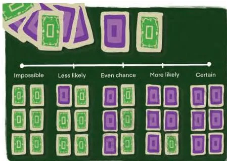
When none of the six cards is purple, picking a purple card is impossible; when all six are purple, it is certain. Between these ends, the probability moves from less likely to even chance to more likely.
Theoretical Probability
When all outcomes are equally likely — no outcome has any reason to be favoured — you do not need an experiment. The theoretical probability of an event \(A\) is the ratio of the outcomes that make \(A\) happen to the total outcomes possible (NCERT, p. 162):
\[ P(A) = \frac{\text{Number of favourable outcomes}}{\text{Number of possible outcomes}} \]
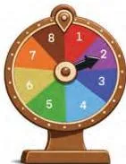
This is what you expect in a perfectly fair situation: a fair coin gives \(P(\text{heads}) = \frac{1}{2}\), and a fair die gives \(P(\text{rolling a 4}) = \frac{1}{6} \approx 0.167\). The spinner below gives another equally likely case — the arrow can stop at any number from 1 to 8.
Experimental Probability
When you actually perform the experiment, or when you work from survey data, count what happened. The experimental probability of an event is (NCERT, p. 161):
\[ P(E) = \frac{\text{Number of times the event occurred}}{\text{Total number of trials}} \]
The same value is called the relative frequency of the event. If a die lands on 3 in 7 out of 40 rolls, the experimental probability is \( \frac{7}{40} = 0.175 = 17.5\% \).
The experimental and theoretical values can differ when trials are few. As trials increase, the experimental probability tends to move closer to the theoretical value — this is the Law of Large Numbers.
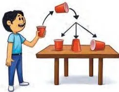
The paper cup is why experimental probability exists: its three landing positions are not equally likely, so you toss it many times and assign probabilities from the results (NCERT, p. 166). The same ratio works for survey data — the class-fruit survey in the textbook gave \( \frac{20}{50} = 0.4 \) for mango (NCERT, p. 163).
Sample Space and Sample Size
The sample space \(S\) is the set of all possible outcomes of a random experiment, and the sample size \(n(S)\) is the number of elements in it (NCERT, p. 167):
\[ S = \{\text{outcome}_1, \text{outcome}_2, \ldots, \text{outcome}_n\}, \quad n(S) = \text{number of elements in } S \]
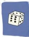
Three rules fix the list: \(S\) must include every possible outcome, no outcome may be listed twice, and \(n(S)\) counts the entries. The coin and the die below give the two most common sample spaces.

| Experiment | Sample space \(S\) | Sample size \(n(S)\) |
|---|---|---|
| Toss a coin | \( \{\text{H}, \text{T}\} \) | 2 |
| Roll a 6-sided die | \( \{1, 2, 3, 4, 5, 6\} \) | 6 |
| Toss two coins | \( \{\text{HH}, \text{HT}, \text{TH}, \text{TT}\} \) | 4 |
Events
An event is one result or a group of results chosen from the sample space — formally, a subset of \(S\) (NCERT, p. 168). Its probability is the theoretical formula with the event’s outcomes counted as favourable. Rolling a die, the event “greater than 4” is \(E = \{5, 6\}\), so \(P(E) = \frac{2}{6} = \frac{1}{3}\).
Tree Diagrams for Multi-step Experiments
A tree diagram lists the outcomes of a multi-step experiment, such as tossing a coin twice or picking one fruit from each of two baskets. Each branch is one possible result, and each path from start to end is one complete outcome (NCERT, p. 169). When all outcomes are equally likely, the probability of any one path is \( \frac{1}{n(S)} \).
For two tosses of a fair coin the tree gives \(S = \{\text{HH}, \text{HT}, \text{TH}, \text{TT}\}\), so:
\[ P(\text{HH}) = \frac{1}{4} = 0.25 = 25\% \]
The event “one head and one tail” covers the paths HT and TH, so its probability is \( \frac{2}{4} = \frac{1}{2} \).
What Each Symbol Means
| Symbol | What it means | Unit / nature |
|---|---|---|
| \(P(E)\) | Probability of event \(E\) | Dimensionless; always between 0 and 1 |
| \(P(A)\) | Theoretical probability of event \(A\) | Dimensionless ratio |
| \(E\), \(A\) | An event: one outcome or a set of outcomes | A subset of the sample space |
| \(S\) | Sample space: set of all possible outcomes | A set |
| \(n(S)\) | Sample size: number of elements in \(S\) | A count (whole number) |
| \(\text{favourable outcomes}\) | Outcomes that make the event happen | A count |
| \(\text{possible outcomes}\) | All outcomes in the sample space | A count |
| \(\text{trials}\) | Number of times the experiment is repeated | A count |
| \(H\), \(T\) | Heads and tails in a coin toss | Outcome labels |
When to Use Each Formula
Chance questions come in two families: those you decide by reasoning and those you decide by data. The chapter-opening situations below — rain, a match result, a lucky draw — are all random: you know the possible outcomes but not which one will occur (NCERT, p. 156).

- Theoretical formula — use when every outcome is equally likely: a fair coin, a fair die, a random card, any draw “without looking”. No experiment data needed (NCERT, p. 160).
- Experimental formula — use when you have trial results or survey data, or when outcomes are not equally likely, as with a paper cup’s landing position. Count events over trials (NCERT, p. 161).
- Probability scale — use to describe an event in words (impossible, less likely, even chance, more likely, certain) and to convert a probability to a percentage by multiplying by 100 (NCERT, p. 158).
- Sample space — write \(S\) first whenever a question says “sample space” or asks for all possible outcomes; check that every outcome appears exactly once (NCERT, p. 167).
- Tree diagram — use for multi-step experiments so no outcome is missed; each path from start to end is one outcome (NCERT, p. 169).
- Law of Large Numbers — use it to explain why the experimental probability differs from the theoretical probability: the gap shrinks as the number of trials grows (NCERT, p. 164).
Worked Examples
The three examples below apply the formulas with fresh numbers. For formula sheets of every class, visit the maths formulas home.
Example 1: Theoretical probability from a word
Step 1: Choose the formula.
A letter is picked at random, so every letter is equally likely.
Use the theoretical formula \(P(A) = \frac{\text{favourable outcomes}}{\text{possible outcomes}}\).
Step 2: Count the outcomes.
The word STATISTICS has 10 letters, so possible outcomes = 10.
The letter S appears 3 times, so favourable outcomes = 3.
\[ P(\text{letter S}) = \frac{3}{10} = 0.3 = 30\% \]
Final answer: \(P(\text{letter S}) = 0.3\), or 30%. It lies inside the 0-to-1 scale, as every probability must.
Example 2: Working backwards from a sample probability
Step 1: The sample probability is an experimental probability.
Suppose 80 students are surveyed and the probability that a randomly chosen student prefers football is 0.35.
Then \(0.35 = \frac{\text{football fans}}{80}\).
Step 2: Multiply the probability by the sample total to obtain the count.
\[ \text{football fans} = 0.35 \times 80 = 28 \]
Final answer: 28 of the 80 sampled students prefer football. Check: \(\frac{28}{80} = 0.35\).
Example 3: Probability from a combined sample space
Step 1: List the sample space.
A coin toss gives \( \{H, T\} \) and a die roll gives the numbers 1 to 6.
Together there are \(2 \times 6 = 12\) equally likely outcomes: \( \{H1, H2, H3, H4, H5, H6, T1, T2, T3, T4, T5, T6\} \).
Step 2: Count the favourable outcomes.
The event “tails and a number greater than 4” contains the outcomes T5 and T6, so favourable outcomes = 2.
\[ P(\text{tails and a number greater than 4}) = \frac{2}{12} = \frac{1}{6} \approx 0.167 \]
Final answer: \(\frac{1}{6}\), about 0.167 or 16.7%.
Common Mistakes to Avoid
| Mistake | Correct rule | How to check your answer |
|---|---|---|
| Using the theoretical formula when outcomes are not equally likely, e.g. a paper cup landing on its bottom, top or side | For outcomes that are not equally likely, use experimental probability from trials or data | Ask: “Is there any reason one outcome is more likely than another?” If yes, you need data, not counting |
| Writing a probability outside 0 to 1, such as \( \frac{3}{2} \) or a negative number | Every probability obeys \( 0 \leq P(E) \leq 1 \); favourable outcomes can never exceed possible outcomes | Your answer is a ratio of two counts — the numerator cannot be larger than the denominator |
| Believing a long run of heads makes tails “due” (gambler’s fallacy) | Each toss is independent; the probability of tails is still \( \frac{1}{2} \) | Remember the coin has no memory — past tosses do not change the next toss |
| Writing the two-coin sample space as \( \{\text{HH}, \text{HT}, \text{TT}\} \) or \( \{H, T\} \), missing a case or merging different outcomes | HT and TH are different outcomes, so \(S = \{\text{HH}, \text{HT}, \text{TH}, \text{TT}\}\) and \(n(S) = 4\) | Draw the tree: every path from start to end is one distinct outcome |
Frequently Asked Questions
What is the difference between theoretical and experimental probability?
Theoretical probability assumes all outcomes are equally likely and uses the formula \( \frac{\text{favourable}}{\text{possible}} \) — it is what you expect in a perfectly fair situation. Experimental probability uses the formula \( \frac{\text{times the event occurred}}{\text{total trials}} \) on data you actually collected.
The two can differ when trials are few; the Law of Large Numbers says they get closer as trials increase (NCERT, pp. 161-162).
Why must every probability lie between 0 and 1?
Because a probability is a ratio of two counts: the favourable outcomes over the possible outcomes. You can never have more favourable outcomes than possible ones, so the ratio can never be below 0 or above 1. The scale runs from 0 (impossible) to 1 (certain) (NCERT, p. 158).
If a coin has shown heads six times, is tails more likely next?
No. This is the gambler’s fallacy. Each toss is an independent event and the coin has no memory, so the probability of tails on the next toss is still \( \frac{1}{2} \) (NCERT, p. 165).
When should I write the sample space first?
Whenever a question says “sample space” or asks for all possible outcomes. Writing \(S\) before calculating also protects you from missing cases. Three checks apply: every possible outcome is included, no outcome appears twice, and \(n(S)\) counts the entries (NCERT, p. 167).
Reference: NCERT Class 9 Mathematics textbook, chapter The Mathematics of Maybe: Introduction to Probability.
Explore Class 9 Maths Formulas
- Previous: Measuring Space: Perimeter and Area
- Next: Predicting What Comes Next: Exploring Sequences and Progressions
More for this chapter:
Class 9 Maths on LearnCBSE:
Related chapters: