These probability class 9 notes rewrite Chapter 7 of the NCERT Ganita Manjari textbook into a short revision form — the probability scale, randomness, sample space, events, the two measurement methods and tree diagrams — with formulas and original worked examples. All page numbers below refer to the NCERT Class 9 book. For the full set of chapter guides, see our Class 9 mathematics notes.
The chapter’s central question is simple: how likely is something to happen? We cannot predict a single coin toss or die roll exactly, but we can measure how likely each result is. That measurement is called probability.
Use the page in this order: read the scale and the two formulas first, then run through the worked examples, then check the common-mistakes table. The revision summary at the end is the compact recap for the night before a test. You can also verify any page against the official PDFs on the NCERT website.
The Probability Scale: From Impossible to Certain
Probability is a measurement of the likelihood of an event, just as length measures size or weight measures heaviness (NCERT, p. 156). It is measured on a scale from 0 to 1. A value of 0.75 means a 75% chance; 0.5 means a 50% chance.
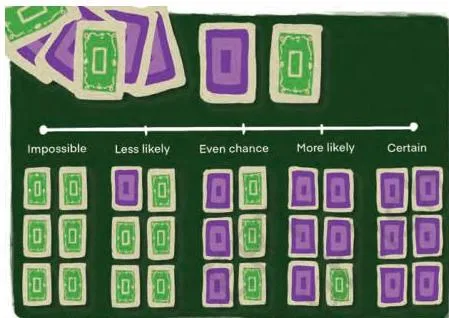
The six-card figure (Fig. 7.1) makes the scale concrete. Imagine a deck of six cards. If none are purple, picking a purple card is impossible (0). If all six are purple, it is certain (1). As purple cards are added, the likelihood moves smoothly from less likely, to even chance, to more likely (NCERT, p. 158).
The book pairs each band with a real event (NCERT, p. 159):
| Event | What it means on the scale |
|---|---|
| Getting a number greater than 6 on a die | Impossible — dice only show 1 to 6 |
| Rolling a 3 on a standard die | Less likely — one face out of six |
| Flipping a coin and getting heads | Even chance — heads and tails equally likely |
| Drawing any card 2 to 10 from a deck of 52 | More likely — 36 such cards exist |
| Choosing a red sweet from an all-red bag | Certain — every sweet is red |
Most real probabilities lie strictly between 0 and 1 — neither impossible nor certain, just more or less likely.
Memory hook: anchor three positions — zero = no way, one = always, one-half = half-and-half (heads or tails). Everything else falls between them.
The whole chapter builds in four stages: the scale, the vocabulary (sample space and events), the two objective measurement methods (experimental and theoretical), and tree diagrams for multi-step experiments. Every section below fits into one of these four stages.
Randomness: Why a Coin Toss Is Unpredictable
Randomness is a situation where you cannot predict the exact result, even though you know every possible result (NCERT, p. 156). In a coin toss you know the outcome is heads or tails, but you cannot say which appears on a single toss.
These repeatable actions are called random experiments or trials. Each observation is an outcome. The lucky-draw example shows the idea: every student’s name is on a slip, one is picked at random, and each student has an equal chance of being chosen.
Randomness extends far beyond coins. Rain depends on temperature, humidity, wind patterns and pressure, so it can never be predicted with total certainty — only its likelihood can be estimated (NCERT, p. 158).
People estimate likelihood in two ways. Subjective probability is a personal guess — a friend sees hot, humid clouds and says rain is likely. The chapter instead teaches objective measurement: collecting evidence, by experiment or reasoning.
Why is a coin toss a fair way to decide who bats first in cricket? Because a fair coin is symmetrical — no side is more likely to land up — so heads and tails are equally likely, each \( \frac{1}{2} \).
Sample Space and Events: The Language of Outcomes
The sample space, written \( S \), is the set of all possible outcomes of a random experiment. Each outcome is an element of the set (NCERT, p. 167).

| Term | Meaning | Example |
|---|---|---|
| Experiment | The random action you repeat | Tossing a coin |
| Outcome | One possible result of the experiment | Heads |
| Sample space \( S \) | Set of all possible outcomes | \( S = \{1, 2, 3, 4, 5, 6\} \) |
| Element | Each individual outcome in \( S \) | The outcome 3 |
| Sample size \( n(S) \) | Number of elements in \( S \) | \( n(S) = 6 \) for a die |
| Event | One result or a group of results chosen from \( S \) | \( E = \{5, 6\} \) for “greater than 4” |
A sample space must obey three rules (NCERT, p. 167):
- It includes every possible outcome.
- No outcome is listed more than once.
- The number of elements is written as the sample size \( n(S) \).
Sample spaces you should know by heart:
- Coin: \( S = \{H, T\} \), \( n(S) = 2 \)
- Die: \( S = \{1, 2, 3, 4, 5, 6\} \), \( n(S) = 6 \)
- Rain: \( S = \{\text{Rain, No Rain}\} \), \( n(S) = 2 \)
- Match: \( S = \{\text{Win, Lose, Draw}\} \), \( n(S) = 3 \)
- Two coins: \( S = \{HH, HT, TH, TT\} \), \( n(S) = 4 \)
The two-coin space is a classic trap. \( HT \) and \( TH \) are different outcomes — the first letter is coin 1 and the second is coin 2, so order matters. The book shows this with a Coin 1 / Coin 2 table (NCERT, p. 167):
| Coin 1 | Coin 2 | Outcome |
|---|---|---|
| H | H | HH |
| H | T | HT |
| T | H | TH |
| T | T | TT |
An event is any single result or combination of results — a subset of the sample space (NCERT, p. 168). Rolling a die, the event “number greater than 4” is \( E = \{5, 6\} \). Picking fruit from a basket with apples, bananas and oranges, the event “a yellow fruit” is \( E = \{\text{Banana}\} \).
Sample spaces can be made more detailed to fit the problem. For rain you may use \( \{\text{Rain, No Rain}\} \), or expand it to \( \{\text{No Rain, Drizzle, Light Rain, Heavy Rain}\} \) when the question cares about rainfall amounts (NCERT, p. 168).
Experimental Probability: Measuring from Real Data
Experimental probability comes from evidence — you perform an experiment or study past data and count how often the event happened. It is also called the relative frequency of the event (NCERT, p. 160).
\[ \text{Experimental Probability} = \frac{\text{Number of times the event occurred}}{\text{Total number of trials}} \]
Original mini-example: roll a die 40 times and a 6 lands 7 times. The experimental probability of rolling a 6 is \( \frac{7}{40} = 0.175 = 17.5\% \). The book’s own example rolls a die 50 times and a 4 lands 8 times, giving \( \frac{8}{50} = 0.16 = 16\% \) (NCERT, p. 161).
The same logic works on existing statistics. In the book’s fruit survey, a class of 50 students is asked for their favourite fruit: 20 say mango, 15 apple, 10 banana, 5 grapes. The probability that a randomly chosen student likes mango is \( \frac{20}{50} = 0.4 = 40\% \) (NCERT, p. 163).
This is a real-life sampling application. The school has 1500 students, but we surveyed only 50. Because the estimate for mango is 0.4, we expect about \( 0.4 \times 1500 = 600 \) students to prefer mango — so we buy roughly 600 mangoes for the school. The 50-student group is the sample; the 1500-student school is the population (NCERT, p. 163).
A larger, more representative sample — say 100 students drawn from several classes — gives a more confident estimate. That is the point of sampling: estimate a big group from a manageable, fair subset.
Theoretical Probability: The Fair-Situation Formula
Theoretical probability assumes all possible outcomes are equally likely — the perfectly fair situation — and reasons about outcomes without doing any experiment (NCERT, p. 162).
\[ P(A) = \frac{\text{Number of favourable outcomes}}{\text{Number of possible outcomes}} \]
Here \( P(A) \) reads “the probability of event A”. Every probability obeys the rule \( 0 \le P(E) \le 1 \).
Why may we assume fairness? A fair coin is symmetrical — no side is heavier or more likely to land up — so it is unbiased. A standard die behaves the same way: each face is equally likely (NCERT, p. 165).
Original example: roll a standard die and find \( P(\text{rolling a 5}) \). Favourable outcomes = 1 (the face 5); possible outcomes = 6; so \( P = \frac{1}{6} \approx 0.167 = 16.7\% \).
The book confirms the same reasoning: \( P(\text{rolling a 4}) = \frac{1}{6} \approx 0.167 \), and a letter picked at random from the word PROBABILITY has \( P(B) = \frac{2}{11} \approx 0.182 \), because two of the eleven letters are B (NCERT, p. 162).
Experimental vs Theoretical: The Law of Large Numbers
The two methods answer the same question from different starting points. This comparison does not appear as a table in the textbook, which explains both in prose — it is worth building yourself:
| Basis | Experimental probability | Theoretical probability |
|---|---|---|
| What it measures | What actually happened in trials or data | What we expect in a fair situation |
| Data needed | Real data — experiments or statistics | None — pure reasoning |
| Core assumption | None | All outcomes equally likely |
| Formula | \( \frac{\text{times event occurred}}{\text{total trials}} \) | \( \frac{\text{favourable}}{\text{possible}} \) |
| When to use | Real counts, surveys, relative frequency | Fair coins, dice, cards |
| Example | Die shows 4 in 8 of 50 rolls: \( \frac{8}{50} = 0.16 \) | \( P(\text{rolling a 4}) = \frac{1}{6} \approx 0.167 \) |
The two can differ, especially when trials are few. The Law of Large Numbers says that as the number of trials grows, experimental probability approaches the theoretical value (NCERT, p. 164). Roll a die 60, then 600, then 6000 times, and the fraction of 3s settles closer and closer to \( \frac{1}{6} \). The pattern stabilises the way sequences and progressions capture regular patterns in numbers.
A common trap follows. After getting heads six times, people expect tails “because it is due”. The coin does not remember — each flip starts afresh, and the probability of tails is still \( \frac{1}{2} \). In Snakes and Ladders, rolling three 6s in a row does not make the fourth roll less likely to be a 6; it stays \( \frac{1}{6} \).
This belief, that past random results change the next one, is called the Gambler’s Fallacy (NCERT, p. 165).
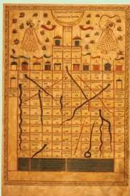
The book’s “Did you know?” note ties this to Indian history: Snakes and Ladders grew out of the ancient Indian dice game Jñān-Chaupad, used to teach moral lessons — ladders for virtues, snakes for vices (Fig. 7.4). Dice games like this are pure random experiments: each roll is independent.
Tree Diagrams: Listing Multi-Step Outcomes
A tree diagram lists all outcomes of a multi-step experiment — a series of independent trials such as tossing a coin twice or rolling a die three times. Each branch carries one possible outcome, and every path from start to end is one complete outcome (NCERT, p. 169).
Toss a fair coin twice. Draw a single point; from it draw one branch to H and one to T (the first toss). From each of H and T draw two more branches, again to H or T (the second toss). The four complete paths are HH, HT, TH and TT, so \( S = \{HH, HT, TH, TT\} \).
Each branch also carries its theoretical probability. \( P(HH) = \frac{1}{4} = 0.25 = 25\% \). The chapter’s Think-and-Reflect asks for the probability of one head and one tail: two of the four paths qualify (HT and TH), so \( \frac{2}{4} = \frac{1}{2} = 0.5 \).
Tree diagrams are visual tools, just like the figures in the measuring space chapter — drawing each step helps you see every combination before you count. Try two comprehension checks from the book (NCERT, p. 169):
- Basket A holds one apple and two oranges; basket B holds one banana and one mango. Pick one fruit from each and draw the tree.
- A box holds 3 red, 4 black and 2 green pens. You pick a pen, put it back, and your friend picks again — draw the tree and find the probability both pick the same colour.
Worked Examples: Step-by-Step Probability
Example 1: A letter is picked at random from the word HARMONY
Method: favourable outcomes over possible outcomes.
Step 1: Count the total letters in HARMONY.
There are 7 letters.
Step 2: Identify the vowels — A and O.
Favourable count = 2.
Step 3: Write the fraction first, then convert:
\[ P(\text{vowel}) = \frac{2}{7} \approx 0.286 = 28.6\% \]
Final answer: \( \dfrac{2}{7} \approx 28.6\% \).
Example 2: A bag has 5 red, 3 blue and 2 green marbles
Method: favourable-over-possible; for “not red”, count the other colours or use \( 1 – P(\text{red}) \).
- Step 1: Total marbles = \( 5 + 3 + 2 = 10 \).
- Step 2: Blue marbles = 3, so
\[ P(\text{blue}) = \frac{3}{10} = 0.3 = 30\% \]
Step 3: Not-red marbles = blue + green = \( 3 + 2 = 5 \), so \[ P(\text{not red}) = \frac{5}{10} = 0.5 = 50\% \]
Check: the complement rule gives the same value: \( 1 – \frac{5}{10} = \frac{5}{10} = 0.5 \).
Final answer: \( P(\text{blue}) = 30\% \), \( P(\text{not red}) = 50\% \).
Example 3: A die is rolled and a coin is tossed together
Method: list the sample space, then favourable-over-possible.
- Step 1: List all 12 outcomes: \( (H,1), (H,2), (H,3), (H,4), (H,5), (H,6), (T,1), (T,2), (T,3), (T,4), (T,5), (T,6) \).
- Step 2: Count the favourable outcomes — an even number \( AND \) a head.
Even die faces are 2, 4, 6, each paired with H: \( (H,2), (H,4), (H,6) \).
So favourable = 3.
Step 3: Possible outcomes = 12.
Write the fraction, simplify, then convert:
\[ P(\text{even and head}) = \frac{3}{12} = \frac{1}{4} = 0.25 = 25\% \]
Final answer: \( \dfrac{1}{4} = 25\% \).
Common Mistakes Students Make in Probability
| Students write | Correct rule | How to check your answer |
|---|---|---|
| \( P(\text{even on a die}) = \frac{3}{5} \) | Correct is \( \frac{3}{6} = \frac{1}{2} \); the possible outcomes are the 6 faces (NCERT, p. 158). | Count every face of the die: 6 possible, 3 even (2, 4, 6). |
| \( P(\text{rolling a 4}) = \frac{6}{1} \) | Correct is \( \frac{1}{6} \); one favourable face out of six (NCERT, p. 162). | Favourable count goes in the numerator, possible count in the denominator. |
| Two-coin space \( \{HH, HT, TT\} \) | Correct is \( \{HH, HT, TH, TT\} \); the coins are different objects, so HT and TH are separate (NCERT, p. 167). | Confirm all four combinations appear exactly once. |
| “Three 6s in a row, so the next must differ” | The probability of a 6 is still \( \frac{1}{6} \); the die has no memory — Gambler’s Fallacy (NCERT, p. 165). | Ask: does the die remember? If not, the probability is unchanged. |
| “\( P = 0.5 \) means it definitely happens” | 0.5 is even chance — equally likely, not certainty; certainty is 1 (NCERT, p. 158). | 0.5 sits at the middle of the scale; 1 means certain. |
Exam Notes: Writing Answers That Earn Marks
This step earns the mark: write the fraction first. In any probability question, show \( \frac{\text{favourable}}{\text{possible}} \) as an unsimplified fraction before converting to a decimal or percentage — the fraction itself usually carries the mark (NCERT, p. 162).
Sample-space answers need braces and commas: write \( S = \{HH, HT, TH, TT\} \), and state the sample size \( n(S) = 4 \) (NCERT, p. 167).
“Not” questions: for “not red”, either count the other colours (blue + green = 5) or use \( 1 – P(\text{red}) \). Both methods must give the same answer — use one to check the other.
Tree diagrams appear for two-step experiments. Label every branch with its outcome and probability; each path from start to end is one complete outcome (NCERT, p. 169).
Always reduce the fraction to lowest terms before converting: \( \frac{3}{12} \) becomes \( \frac{1}{4} \), then write 0.25 or 25%.
These habits run through our Class 9 notes for every subject.
Probability Class 9 Notes at a Glance: Revision Summary
The chapter’s own summary (NCERT, p. 174) lists exactly these bullets — here they are in compact form.
\[ \text{Experimental Probability} = \frac{\text{Number of times the event occurred}}{\text{Total number of trials}} \]
\[ P(A) = \frac{\text{Number of favourable outcomes}}{\text{Number of possible outcomes}} \]
\[ 0 \le P(E) \le 1 \]
| Key fact | Statement |
|---|---|
| Probability scale | 0 = impossible, 1 = certain, \( \frac{1}{2} \) = even chance; most probabilities lie strictly between |
| Sample space | Set of all possible outcomes; must include every outcome, none repeated; size \( n(S) \) |
| Event | A subset of the sample space — one or a group of outcomes |
| Law of Large Numbers | More trials → experimental probability approaches theoretical probability |
| Gambler’s Fallacy | The coin or die has no memory; past results do not change the next probability |
Sample spaces to know by heart:
- Coin: \( \{H, T\} \), \( n(S) = 2 \)
- Die: \( \{1, 2, 3, 4, 5, 6\} \), \( n(S) = 6 \)
- Two coins: \( \{HH, HT, TH, TT\} \), \( n(S) = 4 \)
The one rule to remember: favourable over possible — and write the fraction first. Browse all CBSE notes for the rest of your subjects.
Frequently Asked Questions
What is the difference between experimental and theoretical probability?
Experimental probability uses real data: \( \frac{\text{times the event occurred}}{\text{total trials}} \). Theoretical probability uses reasoning about equally likely outcomes: \( \frac{\text{favourable}}{\text{possible}} \), with no experiment needed. As trials increase, experimental probability approaches the theoretical value (NCERT, p. 164).
Why is probability measured on a scale from 0 to 1 and not 0 to 100?
Probability is a fraction-of-certainty scale: 0 means impossible, 1 means certain, and every event lies between. The 0-to-100 version is just percent form — multiply by 100 to convert, so 0.75 becomes 75% (NCERT, p. 158).
What is the sample space when two coins are tossed together?
It is \( \{HH, HT, TH, TT\} \), with \( n(S) = 4 \). HT and TH are different outcomes because the coins are distinct objects — the first letter is coin 1 and the second is coin 2 (NCERT, p. 167).
After rolling three 6s in a row, is a 6 on the next roll less likely?
No — it stays \( \frac{1}{6} \). The die has no memory of past rolls; this mistaken belief is the Gambler’s Fallacy (NCERT, p. 165).
How do you find the probability of picking a ball that is not red from a bag?
Either count the non-red balls and divide by the total, or use \( 1 – P(\text{red}) \). Both give the same answer — for example, with 5 red in 10 balls, \( 1 – \frac{5}{10} = \frac{5}{10} = 0.5 = 50\% \).
Reference: NCERT Class 9 Mathematics textbook (Ganita Manjari), Chapter 7 — The Mathematics of Maybe: Introduction to Probability.
Explore Class 9 Mathematics Notes
- Class 9 Maths Notes
- Class 9 CBSE Notes
- CBSE Notes for Classes 1 to 12
- Previous: Measuring Space: Perimeter and Area
- Next: Predicting What Comes Next: Exploring Sequences and Progressions
More for this chapter:
Related chapters:
- Orienting Yourself: The Use of Coordinates notes
- Introduction to Linear Polynomials notes
- The World of Numbers notes