
These are the plotting data using matplotlib class 12 notes — the revision notes for Chapter 4, Plotting Data using Matplotlib, from the NCERT Class 12 Informatics Practices textbook, prepared for the 2026-27 session. They compress the whole chapter into the pyplot workflow, the pandas .plot() kinds, the customisation options, chart-by-chart guidance, worked examples and common mistakes.
The chapter turns the results of your pandas and NumPy analysis into charts. When numbers become lines, bars, histograms, scatter plots, box plots or pie charts, variation and relationships between variables become visible at a glance — that is the entire purpose of data visualisation (NCERT, p. 105).
How to use this page: read the chapter map below to see the order of ideas, then jump to the section you need from the table of contents. If you are revising chart types, start at “Chart by Chart”. If you are practising, imitate the three worked examples.
This page is part of the Class 12 Informatics Practices notes series, and everything here follows the NCERT textbook, which you can verify on the official NCERT textbook portal. For other subjects, browse the Class 12 notes index.
How Chapter 4 Builds: From Data to Display
The chapter moves in five blocks. If you already know how DataFrames and NumPy work, skim the first row and start revising from the chart types.
| Chapter block | What it teaches | NCERT pages |
|---|---|---|
| 4.1 Introduction | Why visualise data; definition of data visualisation | 105–106 |
| 4.2 Plotting using Matplotlib | Installing matplotlib, importing pyplot, the first line plot, parts of a figure | 106–108 |
| 4.3 Customisation of Plots | Labels, grids, ticks, markers, colours, linewidth and linestyle | 108–112 |
| 4.4 The Pandas Plot Function | The df.plot() wrapper, the kind values, and six chart types in detail | 112–133 |
| Summary | One-line recaps of the whole chapter | 133–134 |
Notice the build order: pyplot functions come first (plot, show, savefig and the decoration calls), and only then does the chapter show how the same charts are reached through df.plot(kind=…). Each chart type is then explained once on that foundation.
The chapter assumes you already know DataFrames and NumPy from earlier study — revise Data Handling using Pandas I and Data Handling using Pandas II if the examples feel unfamiliar. Other chapters in the same book, such as Internet and Web, are not needed for Chapter 4. A wider collection of CBSE notes for all classes is also available.
Data Visualisation and the Anatomy of a Plot
Data visualisation is the graphical or pictorial representation of data using graphs, charts and similar figures. Its purpose is to reveal variation or show relationships between variables (NCERT, p. 105). Analysis results are usually meant to support a decision; visualisation makes those results understandable quickly.
Matplotlib is Python’s third-party plotting library for this job. Install it once from the command prompt with pip install matplotlib (NCERT, p. 106), then import its plotting module in every program:
import matplotlib.pyplot as plt
plt is only an alias — you may use any name, but plt is the convention. The pyplot module is a collection of functions that create and modify a plot. The central object is the figure: the overall window in which everything is drawn. A figure contains a plotting area, legend, axis labels, ticks and title (NCERT, p. 107).
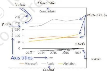
As Figure 4.1 shows, every visible part of a chart has a name: the title names the whole chart, the x and y axis labels say what each axis measures, ticks mark the values along the axes, the legend identifies each plotted series, and the plotting area is where the actual lines, bars or points are drawn.
When you later call plt.title() or plt.xlabel(), you are modifying these very components.
The basic workflow has three steps (NCERT, pp. 107–108):
- Build: plt.plot(x, y) creates the figure — by default a line chart (NCERT, p. 108).
- Display: plt.show() opens a window showing the figure.
- Save: plt.savefig(‘x.png’) writes the current figure to an image file; the save button on the output window does the same (NCERT, p. 108).
The chapter states one rule before any example: always give a chart a title, label its axes, and provide a legend when more than one series is plotted (NCERT, p. 107).
Edge case to remember: if you pass a single list to plt.plot(), Matplotlib treats it as the y values and uses the list index 0, 1, 2, … as x (NCERT, p. 109). This is the answer to the textbook’s first Think and Reflect — to control both axes, pass two equal-length lists.
Plot Customisation Toolkit: Labels, Markers, Colours and Lines
Customisation means changing how a plot looks and what it announces. The chapter groups the options into labelling, markers, colour, linewidth and linestyle.
Labelling functions (NCERT, Table 4.2, pp. 108–109):
| Function | What it does |
|---|---|
| plt.title(‘label’) | Sets a title for the axes |
| plt.xlabel(‘label’) | Sets the label for the x-axis |
| plt.ylabel(‘label’) | Sets the label for the y-axis |
| plt.grid(True) | Configures grid lines in the background |
| plt.xticks(ticks, labels) | Gets/sets tick locations and labels on the x-axis |
| plt.yticks(ticks, labels) | Gets/sets tick locations and labels on the y-axis |
| plt.legend() | Places a legend on the axes |
| plt.show() | Displays all figures |
| plt.savefig(‘x.png’) | Saves the current figure |
Markers: a marker is any symbol that represents a data value in a line chart or a scatter plot (NCERT, p. 110). Common codes are ‘.’ (point), ‘o’ (circle), ‘*’ (star), ‘^’ (triangle up), ‘s’ (square) and ‘D’ (diamond); the full list is in NCERT Table 4.3 (p. 110). Markers are passed to plot() with marker=’*’, and their size is set with markersize.
Colours and lines (NCERT, pp. 110–111):
| Character | Colour |
|---|---|
| ‘b’ | blue |
| ‘g’ | green |
| ‘r’ | red |
| ‘c’ | cyan |
| ‘m’ | magenta |
| ‘y’ | yellow |
| ‘k’ | black |
| ‘w’ | white |
Memory hook: Big Green Rats Can Meet You, King White — the initials B G R C M Y K W are exactly the colour codes. Black is k, not b, because b was already assigned to blue; that is why the mnemonic ends with “King White”.
Linewidth is measured in pixels; the default is 1, so values above 1 give a thicker line. Linestyle takes one of four strings: ‘solid’, ‘dotted’, ‘dashed’ or ‘dashdot’ (NCERT, p. 111). Both are parameters of plot(): linewidth=2, linestyle=’dashed’.
Continuous vs discrete data also drives chart choice (NCERT, pp. 111–112): continuous data is measured and may be decimal — height, weight, temperature; discrete data is obtained by counting and is always a whole number — the number of students in a class. Line charts suit continuous series; counts and categories are usually better as bars.
Pandas .plot(): The Wrapper Behind the Charts
Since pandas version 0.17.0, every Series and DataFrame carries its own .plot() method. It is a wrapper — a thin layer that calls pyplot’s plotting functions for you, using the DataFrame’s columns as the data (NCERT, p. 112). So s.plot() or df.plot() produce the same family of charts as the pyplot functions, with less bookkeeping.
| kind = | Plot type |
|---|---|
| line | Line plot (default) |
| bar | Vertical bar plot |
| barh | Horizontal bar plot |
| hist | Histogram |
| box | Box plot |
| area | Area plot |
| pie | Pie plot |
| scatter | Scatter plot |
(NCERT, Table 4.5, p. 113) plt.plot() vs df.plot() — which one should you use?
| plt.plot() | df.plot(kind=…) | |
|---|---|---|
| Where it lives | matplotlib.pyplot module | Method of Series/DataFrame objects |
| Typical input | Plain lists or NumPy arrays | DataFrame columns |
| Chart type | Line plot by default | Chosen by the kind argument |
| Decorations | plt.title(), plt.xlabel(), plt.ylabel() work with both | |
Use df.plot() when the data already sits in a DataFrame; use plt.plot() or plt.scatter() with plain arrays. Pyplot decoration functions keep working alongside df.plot() — for example, plt.title() still sets the title after a df.plot() call (NCERT, p. 113).
When several columns are plotted, a legend appears by default, associating colours with the plotted data (NCERT, p. 114).
Chart by Chart: What Each kind Is For
Matching the data to the chart type is the first design decision. This table shows the question each chart answers and where the chapter explains it.
| Chart | Question it answers | Typical x data | kind value | Pages |
|---|---|---|---|---|
| Line | How does the value change over time? | Time or continuous data | ‘line’ | 113–116 |
| Bar | How do categories compare? | Category strings | ‘bar’ / ‘barh’ | 116–119 |
| Histogram | How often does each range of values occur? | Continuous values grouped into bins | ‘hist’ | 119–124 |
| Scatter | How are two variables related? | Two measured variables | ‘scatter’ | 124–126 |
| Box | What is the statistical summary, and are there outliers? | Categories with value columns | ‘box’ | 126–130 |
| Pie | What share of the whole does each part hold? | One numeric column; index becomes labels | ‘pie’ | 130–133 |
Line and Bar: Trends and Comparisons
A line plot shows data along a number line and is meant for continuous data; use it to visualise growth or decline over a time interval (NCERT, p. 113). With pandas, df.plot(kind=’line’) uses the DataFrame index as the x-axis because the index is numeric (NCERT, p. 115).
The MelaSales example shows the standard fix. The index runs 0–6, so the ticks are plain numbers — until this swap:
ticks = df.index.tolist()
plt.xticks(ticks, df.Day)
plt.xticks() takes two lists: the tick locations and the labels to place there (NCERT, p. 115). Program 4-5 combines this with per-column colours, marker, markersize, linewidth and linestyle.
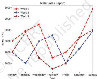
Figure 4.6 is the result: three sales lines, one per week, now labelled Monday to Sunday. The day-name swap is the most common line-plot customisation in this chapter.
A bar chart is the right tool when lines cannot show comparison clearly. Unlike line plots, bar charts can plot strings on the x-axis (NCERT, p. 116). Specify kind=’bar’ and name the column for x: df.plot(kind=’bar’, x=’Day’) (NCERT, p. 117).
If you do not give x, every numeric column of the DataFrame is drawn against the index (NCERT, p. 117). Each column is drawn in its own colour. Bar customisation uses the same parameters as lines: color, edgecolor, linewidth and linestyle (NCERT, p. 118).
For horizontal bars, change kind to ‘barh’ (NCERT, p. 113) — that is also the answer to the textbook’s Think and Reflect about making Figure 4.8 horizontal.
Histograms: Frequencies and Bins
A histogram is a column chart in which each column covers a range of values; the height of a column is the number of data points that fall in that range (NCERT, p. 119). Those ranges are called bins — the intervals into which the data is divided so it can be displayed as bars.
df.plot(kind=’hist’) selects the bins automatically from the spread of the values (NCERT, p. 119). You can also fix them manually with a number, a list of edges, or a range (NCERT, p. 120):
df.plot(kind=’hist’, bins=20)
df.plot(kind=’hist’, bins=[18, 19, 20, 21, 22])
df.plot(kind=’hist’, bins=range(18, 25))
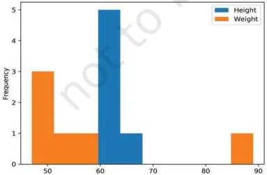
Figure 4.9 shows the plain output of Program 4-8 — a histogram for each numeric column, Height and Weight, with the bins chosen automatically from the data spread.
Histogram customisation: edgecolor (border of each bar), linewidth, linestyle, fill (fill=False leaves the bars empty) and hatch, which fills bars with a pattern such as ‘x’, ‘*’ or ‘o’ (NCERT, p. 120).
Open data context (NCERT, pp. 121–123): open data is data released freely for public download and analysis. The chapter uses the Open Government Data (OGD) Platform India at data.gov.in, where large government datasets are available.
Its temperature example reads only the ‘ANNUAL – MIN’ and ‘ANNUAL – MAX’ columns with the usecols parameter of pd.read_csv(), then plots the frequency of each temperature with ‘Temperature’ and ‘Number of times’ as axis labels.
A frequency polygon can be overlaid on the histogram by computing frequencies and bin edges with np.histogram() and plotting the midpoints of the bins (NCERT, p. 123).
Scatter Plots: Relationships Between Variables
A scatter chart uses dots to represent two variables — one plotted along the x-axis and the other along the y-axis (NCERT, p. 124). Because it shows how two variables move together, a scatter plot is sometimes called a correlation plot (NCERT, p. 124). The size, shape or colour of the dots can carry a third or even a fourth variable.
In the chapter’s discount-versus-sales program, each dot pairs a discount (10% to 50%) with the sales it produced. The customised version adds meaning through size: s=discount*10 makes the bubble ten times the discount value, with color=’red’, marker=’*’ and edgecolor=’blue’ (NCERT, p. 125).
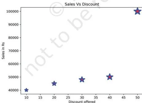
In Figure 4.15, the upward pattern of the stars shows that higher discounts are associated with higher sales, and the larger stars also carry the discount information through their size.
Practical point: plt.scatter() accepts plain array inputs directly, as the program shows with NumPy arrays. df.plot(kind=’scatter’) is meant for DataFrame columns — if your data is only two plain arrays, either build a DataFrame first or stay with plt.scatter().
Box Plots: Quartiles, Whiskers and Outliers
Quartiles are the measures that divide data into four equal parts, each containing the same number of observations (NCERT, p. 126). They are useful whenever data has to be split into groups — for example, finding the top 25 percent of students in an exam.
A box plot is the visual representation of the statistical summary of a dataset: the minimum value, the quartiles, the median and the maximum value (NCERT, p. 126). The whiskers are the two lines outside the box that extend to the highest and lowest values. An outlier is an observation numerically distant from the rest of the data.
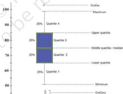
In Figure 4.16, read the five-number summary straight from the drawing: the box carries the quartiles with a median line inside, the whiskers reach the highest and lowest values, and any point standing away from a whisker is an outlier.
A shorter distance between the box and its whiskers means small variation in the data; a longer distance means larger variation (NCERT, p. 128).
With pandas, df.plot(kind=’box’) draws one box per numeric column, which makes it ideal for comparing columns — the Marks.csv example plots one box per subject for a comparative performance analysis (NCERT, p. 127). Add vert=False to draw the boxes horizontally, and change the whisker colour with the color parameter (NCERT, p. 129).
Pie Charts: Proportions of a Whole
A pie chart is a circle divided into sectors, where each sector represents a part of the whole; it represents numerical data proportionally (NCERT, p. 130).
Special rule: df.plot(kind=’pie’) requires either y=’column’ to pick one numeric column, or subplots=True, which draws a separate pie for every numeric column (NCERT, p. 130).
The wedge labels default to the DataFrame index — in the chapter’s planets example, the index values Mercury, Venus and Earth become the labels of the mass pie (NCERT, p. 131).
Pie customisation: explode pulls a wedge outward by a fraction of the radius; autopct=’%.2f’ prints percentage labels on the wedges; colors sets the wedge colours; and legend=False removes the legend (NCERT, pp. 132–133).
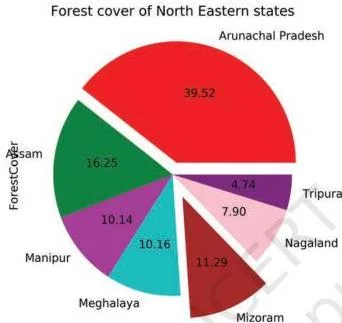
Figure 4.22 is the forest-cover pie after customisation: one wedge is exploded, every sector shows its percentage, and the legend is gone because the state names are already the labels.
Definitions Table: Vocabulary to Write Answers With
These are the terms the chapter expects you to reproduce in short answers. The examples column points to programs already described above.
| Term | Meaning in student words | Example or context |
|---|---|---|
| Data visualisation | Graphical or pictorial representation of data using graphs, charts, etc. | Reveals variation or relationships between variables (NCERT, p. 105) |
| Figure | The overall window where pyplot outputs are plotted | Contains plotting area, legend, axis labels, ticks and title (NCERT, pp. 106–107) |
| Pyplot | The matplotlib module holding functions that create and modify figures | import matplotlib.pyplot as plt (NCERT, p. 106) |
| Marker | Any symbol that represents a data value in a line chart or scatter plot | marker=’*’ in the height-weight line plot (NCERT, p. 110) |
| Legend | The key that identifies which colour or pattern belongs to which series | Appears by default when pandas plots several columns (NCERT, p. 114) |
| Bins | The intervals into which data is divided for a histogram | bins=[18,19,20,21,22] (NCERT, p. 119–120) |
| Quartile | A measure dividing data into four equal parts, each with equal observations | Finding the top 25 percent of students (NCERT, p. 126) |
| Box plot | Visual representation of the statistical summary of data | Subject-wise boxes from Marks.csv (NCERT, p. 127) |
| Whisker | The two lines outside the box extending to the highest and lowest values | Shorter whisker distance = smaller variation (NCERT, p. 128) |
| Outlier | An observation numerically distant from the rest of the data | A point plotted beyond the whisker in a box plot (NCERT, p. 126) |
| Explode | Pulls a pie wedge outward by a fraction of the radius | explode=[0.1,0,0,0,0.2,0,0] in the forest-cover pie (NCERT, p. 132) |
| Autopct | Formats the percentage labels on pie wedges | autopct=’%.2f’ prints percentages with two decimals (NCERT, p. 132) |
| Open data | Data freely available for public download and analysis | data.gov.in, the OGD Platform India (NCERT, p. 121) |
Pyplot Syntax Quick Reference
These are the “formulas” of the chapter — the exact calls you must be able to write.
Pyplot essentials
| Syntax | What it does |
|---|---|
| plt.plot(x, y) | Creates a figure plotting x versus y; line chart by default |
| plt.show() | Displays all figures |
| plt.savefig(‘x.png’) | Saves the current figure to the named file |
| plt.xlabel(‘…’) | Sets the x-axis label |
| plt.ylabel(‘…’) | Sets the y-axis label |
| plt.title(‘…’) | Sets the chart title |
| plt.grid(True) | Adds gridlines to the background |
| plt.xticks(ticks, labels) | Places the given labels at the given tick positions |
pandas df.plot()
| Syntax | What it does |
|---|---|
| df.plot(kind=’line’, color=[‘red’, ‘blue’]) | Line plot, one line per column in its own colour |
| df.plot(kind=’bar’, x=’Day’) | Vertical bar chart with a column on the x-axis |
| df.plot(kind=’barh’) | Horizontal bar chart |
| df.plot(kind=’hist’, bins=20) | Histogram with 20 bins |
| df.plot(kind=’box’) | One box per numeric column |
| df.plot(kind=’pie’, y=’mass’) | Pie chart of one column, y being mandatory or subplots=True |
Chart-specific customisation
| Syntax | What it does |
|---|---|
| plt.scatter(x, y, s=size, color=’red’, marker=’*’, edgecolor=’blue’) | Scatter plot with sized, coloured, star-shaped points |
| df.plot(kind=’box’, vert=False) | Horizontal box plot |
| df.plot(kind=’pie’, y=’ForestCover’, explode=exp, autopct=’%.2f’, colors=c, legend=False) | Pie with explode, percentage labels, colours and no legend |
| df.plot(kind=’hist’, edgecolor=’Green’, linewidth=2, linestyle=’:’, fill=False, hatch=’o’) | Histogram with empty patterned bars |
Remember the two unit-like rules: linewidth is measured in pixels with default 1, and linestyle takes only ‘solid’, ‘dotted’, ‘dashed’ or ‘dashdot’ (NCERT, p. 111).
Worked Examples: From Data to a Finished Plot
Example A: Line Chart of Weekly Library Visitors
Method: line charts suit continuous data over time. Build the plot from two parallel lists, then decorate it.
- Store the days (x-axis) and visitor counts (y-axis) in two lists.
- Call plt.plot(days, visitors, marker=’^’, color=’c’, linestyle=’–‘) so each point carries an upward-triangle marker, the line is cyan and dashed.
- Add the title, axis labels and grid.
- Call plt.show() to display the figure.
import matplotlib.pyplot as plt
days = [‘Mon’, ‘Tue’, ‘Wed’, ‘Thu’, ‘Fri’, ‘Sat’, ‘Sun’]
visitors = [120, 150, 95, 180, 210, 260, 310]
plt.plot(days, visitors, marker=’^’, color=’c’, linestyle=’–‘)
plt.title(‘Weekly Library Visitors’)
plt.xlabel(‘Day’)
plt.ylabel(‘Number of Visitors’)
plt.grid(True)
plt.show()
Output: a cyan dashed line with a triangle marker per day, rising from 120 visitors on Monday to a 310 peak on Sunday — the grid and labels make the growth easy to read.
Example B: Bar Chart of Section-wise IP Averages
Method: a bar chart compares categories, so feed the data through a DataFrame and let one column supply the category names.
- Create a DataFrame with a ‘Section’ column and an ‘Average’ column.
- Call df.plot(kind=’bar’, x=’Section’, y=’Average’) so sections go on the x-axis.
- Set the y-axis label and display.
import pandas as pd
import matplotlib.pyplot as plt
df = pd.DataFrame({‘Section’: [‘A’, ‘B’, ‘C’, ‘D’],
‘Average’: [78, 86, 91, 82]})
df.plot(kind=’bar’, x=’Section’, y=’Average’, title=’Section-wise IP Averages’)
plt.ylabel(‘Average Marks’)
plt.show()
Output: four vertical bars, one per section, with the tallest at Section C (91 average marks); naming x=’Section’ avoids the index-number labels entirely.
Example C: Scatter Plot of Study Hours Against Test Score
Method: a scatter plot shows the relationship between two variables; here the point size also encodes the first variable again (hours), making larger stars represent more study.
- Store hours studied per day and the corresponding test scores.
- Build a sizes list so each point’s area is 20 times the study hours.
- Call plt.scatter(hours, scores, s=sizes, color=’g’, marker=’*’), add labels and title, then show.
import matplotlib.pyplot as plt
hours = [1, 2, 3, 4, 5, 6]
scores = [45, 55, 62, 70, 78, 88] # out of 100
sizes = [h * 20 for h in hours]
plt.scatter(hours, scores, s=sizes, color=’g’, marker=’*’)
plt.title(‘Study Hours vs Test Score’)
plt.xlabel(‘Hours Studied per Day’)
plt.ylabel(‘Test Score’)
plt.show()
Output: green star markers climbing from the bottom left to the top right — a rising trend — with bigger stars for students who studied more hours per day.
Common Mistakes and How to Fix Them
| Mistake | Correct rule | How to check your answer |
|---|---|---|
| Calling df.plot(…) without plt.show() and seeing nothing | df.plot() only builds the figure; always end with plt.show() | Run the script — a figure window must appear at the end |
| Writing color=’b’ expecting black | ‘b’ is blue; black is ‘k’, because ‘b’ is already taken | Recite the colour hook: Big Green Rats Can Meet You, King White |
| Passing one list to plt.plot() and expecting both axes | The single list is treated as y values; x defaults to the index 0,1,2,… | Pass two equal-length lists whenever both axes matter |
| Calling df.plot(kind=’pie’) without y or subplots | A pie needs y=’column’ to pick one numeric column, or subplots=True | Check the call — one of y or subplots=True must be present |
| Calling plt.xticks(labels) with only labels | xticks needs two arguments: tick positions and labels — plt.xticks(ticks, labels) | Count the arguments; positions and labels are both required |
| Reading bins=20 as a bin size of 20 | bins sets the number of intervals (or a list/range of edges), not the width | With bins=[18,19,20,21,22], count the intervals between edges: 4 |
Exam Notes: How to Write a Complete Plotting Answer
Before the plotting questions in the exercise, the textbook prints a standing instruction: “Give appropriate title, set xlabel and ylabel while attempting the following questions” (NCERT, p. 134). Take it literally for every plotting task: set the title with plt.title(), label both axes with plt.xlabel() and plt.ylabel(), and end with plt.show().
For “name the function” questions, give the function name followed by a one-line purpose. savefig() saves the current figure (NCERT, p. 108); legend() identifies the plotted series (NCERT, p. 108) and appears by default when pandas plots several columns (NCERT, p. 114); the box plot is the plot that displays the statistical summary (NCERT, p. 126).
For analysis questions built on a figure, a complete answer reads the values off the chart: state the median from the box line, the highest and lowest values from the whiskers, any outliers as points beyond the whiskers, and compare variation by the whisker distance (NCERT, p. 128).
A description of the chart’s shape alone is incomplete — quote the numbers you actually read.
Revision Summary: One-Line Recaps for the Night Before
Concept → reminder
| Concept | One-line reminder |
|---|---|
| Creating a plot | plt.plot(x, y) builds the figure; the default chart is a line plot |
| Displaying | plt.show() displays every figure — nothing appears without it |
| Saving | plt.savefig(‘x.png’) writes the current figure to a file |
| Decorations | plt.title(), plt.xlabel(), plt.ylabel() and plt.grid(True) are the standard finish |
| Chart type | df.plot(kind=’line’|’bar’|’barh’|’hist’|’box’|’area’|’pie’|’scatter’) |
| One list in plot() | Treated as y values; x defaults to the index 0,1,2,… |
| Histogram bins | Intervals into which data is divided; auto-chosen unless bins= is set |
| Pie rule | df.plot(kind=’pie’) needs y=’column’ or subplots=True |
| Legend | Appears by default when several columns are plotted |
Chart kind → best use → page
| kind | Best used for | NCERT page |
|---|---|---|
| ‘line’ | Continuous data; growth or decline over a time interval | p. 113 |
| ‘bar’ / ‘barh’ | Comparing categories; strings work on the x-axis | p. 116 |
| ‘hist’ | Frequency of values within ranges | p. 119 |
| ‘scatter’ | Relationship between two variables (correlation) | p. 124 |
| ‘box’ | Statistical summary: minimum, quartiles, median, maximum, outliers | p. 126 |
| ‘pie’ | Proportion of a whole | p. 130 |
Frequently Asked Questions
Why does nothing appear when I call df.plot(kind=’line’)?
df.plot() only builds the figure; nothing is drawn on screen until you call plt.show() (NCERT, p. 107). Add plt.show() as the last line of the program. The same rule applies after plt.plot(): build first, display second, and use plt.savefig() if you need an image file.
What is the difference between plt.plot() and df.plot() when creating charts?
plt.plot() is the pyplot function used with plain lists or NumPy arrays, and it draws a line plot by default. df.plot() is a pandas method, available since pandas 0.17.0, that wraps the pyplot function and plots Series and DataFrame columns directly; its kind argument selects the chart type (NCERT, pp. 112–113).
Use df.plot() when your data sits in a DataFrame and plt.plot() or plt.scatter() for plain arrays — you can still decorate either with plt.title(), plt.xlabel() and so on.
How do I choose between a line chart, a bar chart and a scatter plot for a given dataset?
Use a line chart for continuous data or to show growth and decline over time. Use a bar chart to compare categories — bar charts accept strings on the x-axis, which line plots cannot (NCERT, p. 116). Use a scatter plot to show the relationship between two variables, since it is effectively a correlation plot (NCERT, p. 124).
What does the bins parameter actually do in a histogram?
bins sets the intervals into which the data is divided before counting; each column’s height is the number of data points in its bin (NCERT, p. 119). You can pass a single number (bins=20), a list of edges (bins=[18,19,20,21,22]) or a range (bins=range(18,25)). If you omit it, pandas chooses the bins automatically from the spread of the values.
How can I save a Matplotlib plot as an image file?
Call plt.savefig(‘x.png’) with the file name as its argument; the current figure is written to that file (NCERT, p. 108). You can also use the save button on the output window. Saving works alongside plt.show() — call savefig before the program ends.
Why does my pie chart need y= or subplots=True with df.plot(kind=’pie’)?
Because a pie chart draws sectors from one numeric column, so y=’column’ selects that column (NCERT, p. 130). If you only set subplots=True, pandas draws an independent pie for every numeric column. Without one of these, the call has no single column to work with.
Reference: NCERT Class 12 Informatics Practices textbook, chapter Plotting Data using Matplotlib.
Explore Class 12 Informatics Practices Notes
- Class 12 Informatics Practices Notes
- Class 12 CBSE Notes
- CBSE Notes for Classes 1 to 12
- Previous: Data Handling using Pandas – II
- Next: Internet and Web
Related chapters:
- Data Handling Using Pandas – I notes
- Societal Impacts notes
- Project Based Learning notes