
These data handling using pandas ii class 12 notes compress NCERT Class 12 Informatics Practices Chapter 3 (Data Handling using Pandas – II, textbook pages 63-104) into one page you can revise from tonight: every function’s syntax, what it returns, the default behaviours that trip students up, and a clear example for each idea. The notes follow the 2026-27 session.
For the basics — creating a Series and a DataFrame and accessing data from them — revise the Pandas-I notes first; this chapter assumes those.
Everything here uses the same running example as the book — the marksUT table of four students and their scores across the UT1-UT3 rounds (built in Program 3.1) — plus two smaller tables used for reshaping and missing-value work.
Use the jump links to reach the section you need, scan the formula sheet as a final revision pass, and work through the two solved examples at the end: they use completely new numbers, so you can watch the method instead of memorising a printed output.
The official NCERT PDF of this chapter lets you verify every program and output against the source. For the other chapters, the Class 12 Informatics Practices notes hub and the Class 12 hub keep everything indexed.
Chapter Map: What Pandas-II Adds to Your Data Toolkit
One glance at what each block of the chapter does, the functions it introduces, and the pages it covers:
| Topic | What it does | Key functions | Book pages |
|---|---|---|---|
| Descriptive statistics | Summarises each column (or row) with one value | max(), min(), sum(), count(), mean(), median(), mode(), quantile(), var(), std(), describe() | pp. 65-75 |
| Data aggregation | Collapses a set of values into a single summary | aggregate() / agg() | pp. 75-77 |
| Sorting | Orders rows by one or more columns, ascending or descending | sort_values(by, ascending) | pp. 77-78 |
| Group By | Splits rows into groups and computes statistics per group | groupby() with aggregate() / agg() | pp. 79-82 |
| Altering the index | Resets or replaces the row labels | reset_index(), set_index() | pp. 82-84 |
| Reshaping | Changes the row/column arrangement of a table | pivot(), pivot_table() | pp. 84-89 |
| Handling missing values | Finds, drops or fills blank cells | isnull(), any(), dropna(), fillna() | pp. 89-98 |
| MySQL import/export | Moves data between a MySQL database and a DataFrame | create_engine(), read_sql_query(), read_sql_table(), read_sql(), to_sql() | pp. 98-101 |
| Chapter summary | Restates the chapter’s main conclusions | — | pp. 101-102 |
The sections build in a deliberate order. Filtering (Program 3.2) creates the subsets that statistics and aggregation run on; aggregated values then feed group-by, where the same statistic is computed per group. Reshaping reorganises tables so later queries become single calls, and the missing-value and MySQL sections bring real data in and clean it.
Think of the order as: subset → summarise → reorder → regroup → reshape → clean → connect.
Three DataFrames That Run Through the Chapter
Three tables carry almost every example in the chapter. Fix their shapes now so the code later makes sense.
| Table | Rows × columns | What it holds | Used for | Where it appears |
|---|---|---|---|---|
| marksUT (the Program 3.1 table) | 12 × 7 | Scores of Raman, Zuhaire, Ashravy and Mishti in Maths, Science, S.St, Hindi and Eng across UT1, UT2, UT3; Name and UT columns included | Statistics, aggregation, sorting, group by, index work | pp. 64-65, then runs through pp. 65-84 |
| Store sales | 9 × 4 | Sales and profit of stores S1-S4 for 2016, 2017 and 2018 (Total_sales and Total_profit in rupees) | The pivot() examples only; pivot_table() uses the pen-and-colour stock table | Example 3.1, pp. 84-89 |
| UT4 table | 16 × 7 | The same students after a fourth round; Raman has no Maths, Science or Eng score in UT4 (3 NaN cells) | Missing-value detection, dropping and filling | Table 3.2, pp. 90-98 |
Three sliced subsets also appear early — dfUT1, dfUT2 and dfUT3, created by filtering df on the UT column (pp. 82, 66, 78). Notice that a printed slice keeps the parent’s row labels: dfUT1 shows rows 0, 3, 6, 9. That non-continuous index is exactly why the book later introduces reset_index() (p. 83).
Descriptive Statistics: max, min, sum and count
Descriptive statistics summarise the data — methods that give a basic idea about a whole column in one number (NCERT, p. 65). The four workhorses are max(), min(), sum() and count().
| Function | Default (axis=0) | With axis=1 | The trap |
|---|---|---|---|
| max() | Largest value of each column | Highest value in each row | Text columns give the alphabetically last word — max of Name is ‘Zuhaire’ — so use numeric_only=True (NCERT, p. 66) |
| min() | Smallest value of each column | Lowest value in each row | min of Name is ‘Ashravy’; same numeric_only rule (pp. 67-68) |
| sum() | Total of each column | Row total across selected columns | Whole-frame sum concatenates names into ‘RamanRamanRaman…’ — select numeric columns first (NCERT, p. 68) |
| count() | Number of non-NaN values in each column | Number of values in each row | It counts values, not rows: NaN cells are not counted (pp. 69-70) |
The Program 3.2 pattern is filter first, then take the maximum. dfUT2 = df[df.UT == 2] leaves the four UT2 rows; dfUT2.max(numeric_only=True) then returns UT 2, Maths 24, Science 22, S.St 25, Hindi 25, Eng 24 (NCERT, p. 66).
The same filter feeds the row-wise total of Program 3.4: dfRaman[[‘Maths’,’Science’,’S.St’,’Hindi’,’Eng’]].sum(axis=1) gives 102, 104, 95 — Raman’s total across subjects in UT1, UT2 and UT3 (NCERT, p. 69).
Memory aid for axis: axis=0 moves down the rows of a column, so you get one answer per column; axis=1 moves across the row, so you get one answer per row. For every statistical function in this chapter, axis=0 is the default (NCERT, p. 67).
Mean, Median, Mode, Quartiles, Variance and Standard Deviation
These six measures describe the middle and the spread of numeric data. Each pairs with one pandas call.
| Measure | Rule | pandas call | Book page |
|---|---|---|---|
| Mean | Sum of values ÷ count; numeric data only | mean() | p. 70 |
| Median | The middle value; with an even count, the average of the two middle values — scores 20 and 22 give 21 | median() | p. 72 |
| Mode | The most frequent value — Hindi’s 24, scored by three students, is the mode | mode() | pp. 72-73 |
| Quartiles | Cut the data at 25%, 50% and 75%; q=.5 is the median | quantile(q=.25 / .5 / .75) | pp. 73-74 |
| Variance | Average of the squared differences from the mean | var() | p. 74 |
| Standard deviation | Square root of the variance | std() | p. 75 |
| describe() | Prints count, mean, std, min, 25%, 50%, 75% and max for every numeric column in one call | describe() | p. 75 |
Mean is per-column by default; mean(axis=1) on Zuhaire’s sliced rows gives her per-UT averages 20.4, 19.8 and 19.0 (NCERT, p. 71). Note that describe()’s 25%, 50% and 75% rows are exactly the quartiles — the 50% row equals the median.
Data Aggregation: Many Values to One Number
Aggregation transforms a set of values into a single numeric value (NCERT, p. 75). The aggregate functions are the ones you just met — max(), min(), sum(), count(), std(), var() — and the tool is aggregate(), with agg() as its interchangeable alias (NCERT, p. 81).
- One function on the whole table: df.aggregate(‘max’) returns the maximum of every column, Name included (pp. 75-76).
- Several functions in one call: df.aggregate([‘max’,’count’]) returns one row per function (p. 76).
- One column: df[‘Maths’].aggregate([‘max’,’min’]) returns max 24 and min 12 (p. 76).
- Row-wise: df[[‘Maths’,’Science’]].aggregate(‘sum’, axis=1) totals both subjects for each row — same axis rule as max() and sum() (pp. 76-77).
The default axis is 0, so aggregation is column-wise; passing axis=1 aggregates rows instead.
Sorting a DataFrame: sort_values() in Action
Syntax on p. 77: DataFrame.sort_values(by, axis=0, ascending=True). by is the column or list of columns to sort on, axis=0 means sort the rows, and ascending=False gives descending order.
- Whole table by name: df.sort_values(by=[‘Name’]) — alphabetical, ascending by default (NCERT, p. 77).
- Descending: dfUT3.sort_values(by=[‘Eng’], ascending=False) — English scores in UT3, highest first (Program 3.9, p. 78).
- Multi-column tie-break: dfUT3.sort_values(by=[‘Science’,’Hindi’]) — Zuhaire and Mishti both scored 18 in Science, so pandas uses Hindi to order them; Mishti (25) follows Zuhaire (23) (pp. 78-79).
sort_values() returns a new DataFrame. The original keeps its row order unless you assign the result or pass inplace=True.
Group By: The Split-Apply-Combine Strategy
Group By answers one statistic per group of rows: average Maths per student, total sales per store. It follows a three-step split-apply-combine strategy (NCERT, p. 79). Figure 3.1 is the book’s working picture of the idea.
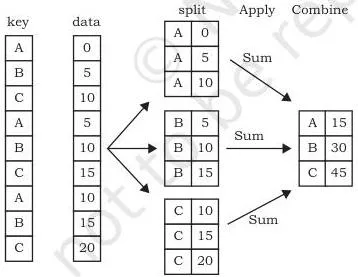
Reading the diagram with the three steps: the two-column (key, data) DataFrame is split so that rows sharing key A form one group, key B another and key C another; sum() is applied inside each group; and the three single results are combined into a new DataFrame — one row per key.
Everything else in this section is pandas syntax for those three steps.
- Create the group object: g1 = df.groupby(‘Name’). The method is the lowercase groupby() — the book’s running text writes GROUP BY, but the Python call is df.groupby(…) (pp. 79-80).
- Helpers on the group object: g1.first() shows the first row of each group; g1.size() the group sizes (3 for each student here); g1.groups a dictionary mapping each name to its row indexes; g1.get_group(‘Raman’) returns only Raman’s three rows (NCERT, p. 80).
- Two attributes at once: df.groupby([‘Name’,’UT’]) groups by both columns (pp. 80-81).
- Grouped aggregation — step 2 of the strategy: df.groupby([‘UT’]).aggregate(‘mean’) gives one row per UT with the subject averages; group1 = df.groupby([‘UT’]) then group1[‘Maths’].aggregate(‘mean’) restricts it to one column (NCERT, p. 81).
- Program 3.10: df.groupby(by=’Name’)[‘Maths’].agg([‘mean’,’var’,’std’,’quantile’]) builds a full per-student summary table in one call (NCERT, p. 82).
One misconception to clear: the group object alone is only the split (step 1). Nothing is computed until you apply a function — that is why the helpers and aggregations above exist.
Altering the Index: reset_index() and set_index()
The default index is a numeric label starting at 0 for each row (p. 82). Slicing copies the parent’s labels, so dfUT1 = df[df.UT == 1] prints rows 0, 3, 6, 9 — a non-continuous index (pp. 82-83). The book fixes it in four moves:
- dfUT1.reset_index(inplace=True) — adds a fresh continuous 0-3 index and stores the old labels in a new ‘index’ column (NCERT, p. 83).
- dfUT1.drop(columns=[‘index’], inplace=True) — removes that leftover column (p. 83).
- dfUT1.set_index(‘Name’, inplace=True) — promotes the Name column to be the row index (pp. 83-84).
- dfUT1.reset_index(‘Name’, inplace=True) — restores the integer index (NCERT, p. 84).
Each call needs inplace=True for the change to be saved on the original variable. Without it, pandas returns a modified copy that nobody keeps.
Reshaping Data: pivot() and pivot_table()
Reshaping changes the arrangement of rows and columns to make a question easier to answer (NCERT, p. 84). The chapter’s example is nine rows of store sales: S1-S4 across 2016-2018 (Example 3.1, pp. 84-85).
Before reshaping, answering questions means slicing store by store: total sales of S1 needs four filter-and-sum blocks for the ‘which store sold most overall’ question (NCERT, p. 85). After pivoting, the same queries become one-liners:
- pivot1 = df.pivot(index=’Store’, columns=’Year’, values=’Total_sales(Rs)’) — stores become rows, years become columns, and missing combinations (S2 in 2016, S4 in 2017 and 2018) become NaN (pp. 85-86).
- pivot1.loc[‘S1’].sum() now answers the total; pivot1.loc[‘S3’].max() the best single year (NCERT, p. 86).
- Multiple values are allowed: values=[‘Total_sales(Rs)’,’Total_profit(Rs)’] (NCERT, p. 87).
Every (index, column) pair inside pivot() must be unique. With the chapter’s pen-and-colour table — two Red Pens exist — df.pivot(index=’Item’, columns=’Color’, values=’Units_in_stock’) fails with the exact message: ‘ValueError: Index contains duplicate entries, cannot reshape’ (pp. 87-88). Recognise that sentence; it names the whole problem.
pivot_table() is pivot() plus aggregation: duplicate rows are combined by aggfunc, whose default is mean (NCERT, p. 88). Syntax: pandas.pivot_table(data, values=None, index=None, columns=None, aggfunc=’mean’).
- Multiple aggregates: aggfunc=[sum, max, np.mean] (pp. 88-89).
- Different functions per column: aggfunc={‘Price(Rs)’:len, ‘Units_in_stock’:np.mean} (pp. 88-89).
- Program 3.11: dfpen.pivot_table(index=’Item’, columns=[‘Color’], values=[‘Price(Rs)’], aggfunc=[max]) prints the maximum pen price per colour (NCERT, p. 89).
The one-line comparison: pivot() reshapes only and refuses duplicate pairs; pivot_table() reshapes and aggregates the duplicates, by mean unless you change aggfunc.
Handling Missing Values: Check, Drop or Fill
A missing value, denoted NaN, is a cell with no value — an unfilled survey field or an attribute that does not apply to that row (NCERT, p. 89). The chapter’s running story (pp. 90-91): after UT4, Raman has no Maths, Science or Eng score. Three teachers handle the same gap three different ways, and each way is a real missing-value strategy.
| Situation / teacher’s decision | pandas tool | What happens | Percentage in the book |
|---|---|---|---|
| No gap — Hindi has all four scores | — | The calculation uses all four rounds | Hindi: 84% (p. 94) |
| Missing score left unfilled | sum() skips the NaN but the formula still divides by four rounds of 25 | The gap pulls the percentage down | Maths: 57% (p. 94) |
| Maths teacher drops that round | dropna() | Raman’s fourth row is removed; only three rounds remain | Maths: 76% (p. 96) |
| Science teacher awards zero | fillna(0) | The missing cell becomes 0 | Science: 60% (pp. 96-97) |
| English teacher repeats the previous round’s mark | fillna(method=’pad’) | The UT4 cell takes UT3’s value | Eng: 91% (p. 97) |
Checking tools come first, in this order:
- df.isnull() — True/False for every cell (p. 91).
- df[‘Science’].isnull() — per-cell check of one column (NCERT, p. 92).
- df.isnull().any() — which columns contain at least one NaN (pp. 92-93).
- df.isnull().sum() — the count of NaN per column (Maths 1, Science 1, Eng 1); add another .sum() to get the table-wide total of 3 (NCERT, p. 93).
Then the two families of fixes. dropna() removes whole rows, which shrinks the data; it suits cases where few objects are affected — dfRaman.dropna(inplace=True, how=’any’) leaves three rows (pp. 94-96). fillna() replaces values: a constant like fillna(0), or a neighbour — method=’pad’ copies the previous value and method=’bfill’ copies the next one (pp. 96-97).
Two edge cases the book leaves implicit. First, pad (and bfill) need a neighbour: if the first cell of a column is NaN, pad has no earlier value to copy, so that gap stays NaN. Second, count() excludes NaN entirely — a 12-row column with 3 missing cells reports 9.
The book is honest about the cost: any estimation changes the data, so results after filling are good approximations, not the original values (NCERT, p. 98).
The chapter’s closing activity applies exactly these skills to the public auto-mpg data from the UCI repository (p. 104) — two of its exercises ask you to replace missing values with the value before them and to remove rows that contain missing values.
Import and Export of Data between Pandas and MySQL
Real data usually lives in files or databases, not in typed-out Python lists (NCERT, p. 98). To move data between MySQL and pandas you need exactly three pieces:
- Install the two libraries: pip install pymysql (the database driver) and pip install sqlalchemy (the library that manages the connection) (pp. 98-99).
- Create an engine: engine = create_engine(‘mysql+pymysql://username:password@host:port/name_of_database’) — this returns the engine object that every read/write call receives (NCERT, p. 99). The connection string carries the driver (mysql+pymysql), the username (normally root), the password, the host (usually localhost), the port (3306 is the default) and the database name.
- Read or write using that engine.
Reading a table into a DataFrame uses three functions (pp. 99-100): pd.read_sql_query(query, engine) for a SELECT statement, pd.read_sql_table(table_name, engine) for a whole table, and pd.read_sql(sql, engine) which accepts either.
Writing uses df.to_sql(table, engine, if_exists=’fail’, index=False). The if_exists parameter decides what happens when the table already exists:
| if_exists value | Behaviour |
|---|---|
| ‘fail’ | Default; raises a ValueError if the table already exists (NCERT, p. 100) |
| ‘replace’ | Overwrites the previous contents (p. 100) |
| ‘append’ | Adds rows to the existing table, whose column sequence must match (p. 100) |
index=False keeps the DataFrame index out of the MySQL table (NCERT, p. 101). The book demonstrates the whole round-trip with the CARSHOWROOM database and its INVENTORY table from Chapter 1, then exports a small table named showroom_info back to MySQL (pp. 99-101).
Key Terms and Definitions at a Glance
| Term | Meaning | Example from this chapter |
|---|---|---|
| Descriptive statistics | Methods that summarise data so you get a basic idea of it in one glance (p. 65) | df.max() returning the largest value of each column |
| axis | The direction pandas steps through the table: 0 goes down each column (default), 1 goes across each row (p. 67) | df.max(axis=1) giving every student’s highest score across subjects |
| numeric_only | Parameter that restricts a statistic to numeric columns (p. 66) | df.max(numeric_only=True) skipping the Name column |
| Aggregation | Collapsing a set of values into a single summary value (p. 75) | df.aggregate(‘max’) |
| Aggregate function | The function applied during aggregation: max, min, sum, count, std, var (p. 75) | df[‘Maths’].aggregate([‘max’,’min’]) |
| Group by object | The result of df.groupby(…); it organises rows into split groups (p. 80) | g1 = df.groupby(‘Name’), then g1.groups |
| Split-apply-combine | The three-step strategy of group by: split into groups, apply a function, combine results (p. 79) | Split by UT, apply mean(), combine into per-UT averages |
| Index (row label) | The labels attached to rows, used for fast access (p. 82) | Default numeric 0-11; changed to names by set_index(‘Name’) |
| Reshaping | Changing the arrangement of rows and columns to make analysis easier (p. 84) | Pivoting store sales so each store becomes a row |
| NaN / missing value | A cell without a value, denoted NaN (p. 89) | Raman’s missing Maths score in UT4 (p. 91) |
| Connection string | The single text carrying driver, user, password, host, port and database to create_engine() (p. 99) | mysql+pymysql://root:password@localhost:3306/CARSHOWROOM |
| Engine object | Returned by create_engine(); handed to every read and write function (p. 99) | engine = create_engine(…) then pd.read_sql_query(query, engine) |
| if_exists | The to_sql parameter that decides what happens when the target table already exists (p. 100) | if_exists=’replace’ overwrites; ‘append’ adds rows |
| inplace | Whether a method modifies the original DataFrame (True) or returns a copy (False) (p. 83) | reset_index(inplace=True) changing dfUT1 permanently |
Formula Sheet: The Statistics That Appear in This Chapter
| Quantity | Rule / formula | pandas function | Page |
|---|---|---|---|
| Mean | \( \text{Mean} = \frac{\text{sum of values}}{\text{number of values}} \) | mean() | p. 70 |
| Median | Middle value; even count → average of the two middles, e.g. \( \frac{20+22}{2} = 21 \) | median() | p. 72 |
| Mode | Most frequent value | mode() | p. 72 |
| Quartiles | \( q=.25 \) (25%), \( q=.5 \) (median), \( q=.75 \) (75%) | quantile(q=…) | pp. 73-74 |
| Variance | Average of the squared differences from the mean | var() | p. 74 |
| Standard deviation | \( \sqrt{\text{variance}} \) | std() | p. 75 |
| Percentage of scores (Programs 3.12-3.13) | \( \frac{\text{sum of scores} \times 100}{25 \times \text{number of UT rounds}} \) | Manual: dfHindi.sum()*100/(25*row) | pp. 93-94 |
| describe() band | count, mean, std, min, 25%, 50%, 75%, max | describe() | p. 75 |
| Connection string | driver://username:password@host:port/database | create_engine() | p. 99 |
Remember that describe()’s 25% / 50% / 75% rows are the quartiles — the 50% row equals the median.
Worked Examples: A Fresh DataFrame, Solved Step by Step
Both examples below use completely new numbers — no marksUT scores, no store sales figures — so you can watch the method instead of memorising an output. Every step states the call, then shows what it returns, with a note on data types where they change.
Worked Example 1: Assignment Scores — Statistics and Aggregation
Method: build a DataFrame from a dictionary, then apply descriptive statistics and aggregation one call at a time.
Step 1 — create the DataFrame. Four students (Kiran, Meera, Arjun, Divya) took three assignments (Asst 1-3), each scored on three components: MCQ, Written and Viva. Meera’s first Viva mark is left as np.nan.
| Name | Asst | MCQ | Written | Viva |
|---|---|---|---|---|
| Kiran | 1 | 15 | 9 | 6.0 |
| Kiran | 2 | 17 | 10 | 7.0 |
| Kiran | 3 | 19 | 11 | 8.0 |
| Meera | 1 | 14 | 12 | NaN |
| Meera | 2 | 16 | 10 | 7.0 |
| Meera | 3 | 18 | 11 | 6.0 |
| Arjun | 1 | 16 | 10 | 5.0 |
| Arjun | 2 | 18 | 12 | 6.0 |
| Arjun | 3 | 20 | 11 | 8.0 |
| Divya | 1 | 17 | 11 | 7.0 |
| Divya | 2 | 19 | 13 | 8.0 |
| Divya | 3 | 21 | 12 | 9.0 |
Data-type note: the MCQ and Written columns are int64, but Viva is float64 — a column that holds even one NaN cannot stay int64.
Step 2 — column-wise maxima. dfA.max(numeric_only=True) returns Asst 3, MCQ 21, Written 13, Viva 9. Without numeric_only, the Name column would also appear — and its maximum would be ‘Meera’, the alphabetically last name.
Step 3 — column-wise means. dfA.mean() returns Asst 2.0, MCQ 17.5, Written 11.0, Viva 7.0. The Viva mean is computed over the 11 present values only — pandas skips the NaN by default.
Step 4 — row-wise totals. dfA[[‘MCQ’,’Written’,’Viva’]].sum(axis=1) gives 30, 34, 38, 26, 33, 35, 31, 36, 39, 35, 40, 42. Meera’s first assignment totals 26 because the NaN contributes nothing. Filling it with fillna(0) first gives the same total — the difference would appear only in the next step.
Step 5 — row-wise means. dfA[[‘MCQ’,’Written’,’Viva’]].mean(axis=1) gives 10.0, 11.33, 12.67, 13.0, 11.0, 11.67, 10.33, 12.0, 13.0, 11.67, 13.33, 14.0 (rounded to 2 d.p.). Meera’s first row is 13.0 because mean() divides by the 2 present values; with fillna(0) that row would be 26 ÷ 3 = 8.67. Same total, different mean — that is why the choice of missing-value strategy matters.
Step 6 — aggregation on one column. dfA[‘MCQ’].agg([‘max’,’min’]) returns max 21 and min 14.
Worked Example 2: One Small Pipeline — Sort, Group, Fill, Pivot
Method: combine the later skills into one mini analysis on the same DataFrame: filter, multi-column sort, grouped aggregation, a padded fill, and a final reshape.
Step 1 — multi-column sort with a tie-break. First filter to Asst 2, then sort it: dfA2 = dfA[dfA.Asst == 2]; dfA2.sort_values(by=[‘Written’,’MCQ’]).
| (index) | Name | Asst | MCQ | Written | Viva |
|---|---|---|---|---|---|
| 4 | Meera | 2 | 16 | 10 | 7.0 |
| 1 | Kiran | 2 | 17 | 10 | 7.0 |
| 7 | Arjun | 2 | 18 | 12 | 6.0 |
| 10 | Divya | 2 | 19 | 13 | 8.0 |
Meera and Kiran tie on Written 10, so MCQ breaks the tie: 16 before 17. Notice the original indexes 1, 4, 7, 10 ride along — the same non-continuous index effect that motivates reset_index() in the book.
Step 2 — grouped aggregation. dfA.groupby(‘Name’)[‘MCQ’].mean() returns Kiran 17.0, Meera 16.0, Arjun 18.0, Divya 19.0 — one clean statistic per student.
Step 3 — locate the gap. dfA.isnull().sum() reports Name 0, Asst 0, MCQ 0, Written 0, Viva 1 — the single missing cell is in Viva.
Step 4 — pad the missing value. The Viva column starts 6, 7, 8, NaN, … ; dfA[‘Viva’].fillna(method=’pad’) turns the NaN into 8.0, copying the previous row. Two honest caveats: pad borrows the previous row of the column (here Kiran’s 8, since the rows are ordered by student) — the book’s English example works cleanly because only Raman’s rows were selected first.
And if the very first cell were NaN, pad would have no earlier value and would leave it unfilled — use bfill or a constant for a leading gap.
Step 5 — reshape with pivot_table. dfA.pivot_table(index=’Name’, columns=’Asst’, values=’MCQ’, aggfunc=’max’) puts each student on a row and each assignment in a column:
| Asst | 1 | 2 | 3 |
|---|---|---|---|
| Kiran | 15.0 | 17.0 | 19.0 |
| Meera | 14.0 | 16.0 | 18.0 |
| Arjun | 16.0 | 18.0 | 20.0 |
| Divya | 17.0 | 19.0 | 21.0 |
Every (Name, Asst) pair here is unique, so the max of a single value is just that value — pivot() would also work. In a table with duplicate pairs, pivot() would raise the duplicate-entries error and pivot_table() would aggregate them with aggfunc instead.
Step 6 — what the reshape now answers easily. With Name as the row index and Asst as columns, each student’s progress across assignments is one row: compare columns 1, 2, 3 to see who improved most — Divya’s 17 → 19 → 21 is the clearest rise.
Mistakes Students Make in This Chapter — and the Corrections
| Students write / do | Correct version | Why |
|---|---|---|
| df.max() returns ‘Zuhaire’ from the Name column | df.max(numeric_only=True) | Text columns compare alphabetically, so the largest Name is the last one in the dictionary order (NCERT, p. 66) |
| Thinking axis=0 means rows | In max()/sum()/mean(), axis=0 is column-wise (default); axis=1 is row-wise | The axis memory aid: axis=0 moves down the rows of a column (NCERT, p. 67) |
| df.sum() on the whole frame prints ‘RamanRamanRaman…’ | Select numeric columns first: df[[‘Maths’,’Science’,…]].sum() | sum() concatenates text strings when they appear in the frame (NCERT, p. 68) |
| Calling sort_values() and seeing no change | Assign the result, or pass inplace=True | sort_values() returns a new DataFrame; the original keeps its order (p. 77) |
| Writing df.GROUP BY(‘Name’) | df.groupby(‘Name’) | The Python method is the lowercase groupby(); GROUP BY is only the textbook’s descriptive name (pp. 79-80) |
| pivot() on data with duplicate index-column pairs | Use pivot_table() instead | pivot() raises ‘ValueError: Index contains duplicate entries, cannot reshape’; pivot_table() aggregates the duplicates with aggfunc, default mean (pp. 87-88) |
| dropna() appears to do nothing | df.dropna(inplace=True) or df = df.dropna() | Without inplace, a modified copy is returned and thrown away (p. 95) |
| Expecting count() to count rows even when cells are blank | count() counts non-NaN values only | A 12-row column with 3 NaN reports 9, not 12 (pp. 69-70) |
| fillna(method=’pad’) leaves the first cell NaN | Use method=’bfill’ for a leading gap, or a constant | pad needs an earlier value; a leading gap has none (p. 97 — the book leaves this edge case implicit) |
| to_sql raises ValueError on an existing table | Pass if_exists=’replace’ or if_exists=’append’ | The default if_exists=’fail’ deliberately refuses to overwrite an existing table (pp. 100-101) |
How to Write Complete Answers to the Chapter Exercises
The chapter exercises sit on pp. 102-104. Read them by question family, and match the length of your answer to what each family demands.
(a) Install-command questions (Q1). A complete answer is one line: pip install pymysql. If asked about the connection library as well, add pip install sqlalchemy (pp. 98-99).
(b) Difference questions (Q2, Q11). Use the two-part structure: define each thing, then state the decisive difference. For pivot() versus pivot_table(): pivot() reshapes only and fails on duplicate index-column pairs; pivot_table() aggregates the duplicates with aggfunc, whose default is mean (pp. 87-88).
For the importance of reshaping (Q11): define shape as the row/column arrangement, then contrast the store-sales questions — four filter-sum blocks before, single pivot1.loc[] calls after (pp. 84-86).
(c) Definition questions (Q3, Q5, Q6, Q7, Q8, Q12). Give the statistical or technical definition, the formula where one exists, and the pandas function name. Median: the middle value; with an even count, the average of the two middles — 20 and 22 give 21 (p. 72). Mode: the most frequent value, found with mode() (p. 72).
Variance: the average of squared differences from the mean, found with var() (p. 74). Standard deviation: the square root of the variance, found with std() (p. 75). Missing values: cells with no value, denoted NaN; strategies are dropping the row or filling with an appropriate value (pp. 89-90, 96). sqlalchemy: the library that manages the connection between Python and MySQL (pp. 98-99).
(d) Code-writing questions (Q13, Q14, pp. 103-104). Use a fixed skeleton: import pandas as pd, and numpy as np wherever a NaN value must be created; build the DataFrame with pd.DataFrame({…}); then write one statement per sub-part, naming the required method and its parameters — numeric_only, axis, ascending, inplace, set_index, groupby(…).aggregate(…), pivot_table, sort_values, fillna, to_sql.
The book’s own programs are the best template: each output is preceded by a printed heading string.
(e) MySQL steps (Q10, and the MySQL parts of Q13). Give a short ordered list: install pymysql and sqlalchemy; create the engine with create_engine(‘mysql+pymysql://user:password@host:3306/database’); then read with read_sql_query or read_sql_table, or write with to_sql (pp. 99-101).
Revision Recap: One-Page Function Cheat Sheet
First, the task-to-function map — if you can name the question, this table names the tool:
| Analysis question | Best tool |
|---|---|
| Largest / smallest value in each column, numbers only | max() / min() with numeric_only=True |
| Add up a column, or a row | sum() with the right axis (0 or 1) |
| Typical value of a column | mean() for the average, median() for the middle value |
| Value that appears most often | mode() |
| How spread out the values are | var() and std() |
| Every column summary at once | describe() |
| Several summaries in one call | aggregate([‘max’,’count’]) |
| Reorder rows by one or more columns | sort_values(by=[…]) |
| The same statistic for each group of rows | groupby(‘key’).aggregate(‘mean’) — grouped aggregation |
| Reshape long data into a cross-tab | pivot() when pairs are unique; pivot_table() when duplicates may exist |
| Locate the blank cells | isnull() with any() / sum() |
| Remove rows with blanks | dropna(inplace=True) |
| Replace blanks | fillna(value), or fillna(method=’pad’ / ‘bfill’) |
Now the master function table, with defaults:
| Function | What it does | Key parameters / defaults | Page |
|---|---|---|---|
| max() / min() | Largest / smallest value per column (axis=0) or row (axis=1) | numeric_only=True to skip text columns | pp. 66-68 |
| sum() | Total per column or row | axis=0 default; select numeric columns first | pp. 68-69 |
| count() | Number of non-NaN values per column / row | axis=1 counts across rows | pp. 69-70 |
| mean() | Average; numeric columns only | Skips NaN; per-row with axis=1 | pp. 70-71 |
| median() | Middle value | Even count → mean of the two middle values | p. 72 |
| mode() | Most frequent value | Can return more than one row | pp. 72-73 |
| quantile(q=.25 / .5 / .75) | Quartiles | q=.5 equals the median | pp. 73-74 |
| var() | Average of squared differences from the mean | — | p. 74 |
| std() | Square root of variance | — | p. 75 |
| describe() | count, mean, std, min, 25%, 50%, 75%, max in one table | Numeric columns | p. 75 |
| aggregate() / agg() | One or several summaries in one call | axis=0 default; agg() is the alias | pp. 75-76, 81 |
| sort_values(by, ascending=True) | Orders rows by column(s) | by accepts a list; returns a new DataFrame | p. 77 |
| groupby(‘key’) | Splits rows into groups | Pair with .first(), .size(), .get_group(), .aggregate() | pp. 79-82 |
| reset_index() | Rebuilds a continuous index | inplace=True to save; old labels kept as a column | pp. 83-84 |
| set_index(‘col’) | Promotes a column to the index | inplace=True to save | pp. 83-84 |
| pivot(index, columns, values) | Reshapes long data wide | Fails on duplicate pairs | pp. 85-88 |
| pivot_table(…, aggfunc=’mean’) | Reshapes and aggregates duplicates | aggfunc can be a list or a dict | pp. 88-89 |
| isnull() | True wherever a cell is missing | Chain .any() or .sum() | pp. 91-93 |
| dropna() | Removes rows containing NaN | inplace=True; how=’any’ drops on any NaN | pp. 94-96 |
| fillna(value) | Replaces NaN with a constant | method=’pad’ / ‘bfill’ for neighbour values | pp. 96-97 |
| create_engine(conn_string) | Opens a MySQL connection | Returns the engine object | p. 99 |
| read_sql_query / read_sql_table / read_sql | Reads a query or whole table into a DataFrame | All take the engine object | pp. 99-100 |
| to_sql(table, conn, if_exists=’fail’, index=…) | Writes the DataFrame to a MySQL table | ‘fail’ / ‘replace’ / ‘append’ | pp. 100-101 |
The whole chapter in five sentences:
- axis=0 is column-wise by default for every statistic in this chapter; axis=1 flips it to row-wise.
- Grouping is split-apply-combine: groupby() splits, an aggregation applies, and pandas combines the group results.
- pivot() reshapes but refuses duplicate pairs; pivot_table() reshapes and aggregates them instead, by default with mean.
- Find gaps with isnull(); then either dropna() the rows or fillna() with a constant, the previous value (pad) or the next value (bfill).
- MySQL access needs pymysql and sqlalchemy, an engine from create_engine(connection-string), then read_sql_query / read_sql_table / read_sql for reading and to_sql for writing.
For the other chapters, browse the Class 12 Informatics Practices hub and the companion plotting data using Matplotlib notes for visualising the DataFrames you clean here. Everything for the class sits in the Class 12 hub, inside the complete CBSE notes library.
FAQs: Doubts Students Ask About Pandas-II
What is the difference between agg() and aggregate() in pandas?
There is no functional difference: agg() is simply a shorter alias for aggregate(). The book states that aggregation can be performed using either name (NCERT, p. 81).
Both take a function name or a list of function names and apply them to columns by default (axis=0) — so df[‘Maths’].aggregate([‘max’,’min’]) and df[‘Maths’].agg([‘max’,’min’]) are the same call.
When should I use pivot_table() instead of pivot()?
Use pivot_table() whenever the data may contain duplicate (index, column) pairs. pivot() demands one unique value per pair and raises ‘ValueError: Index contains duplicate entries, cannot reshape’ when duplicates exist (pp. 87-88). pivot_table() handles the duplicates by aggregating them with aggfunc, whose default is mean (NCERT, p. 88).
If your pairs are guaranteed unique, pivot() works and returns the values unchanged.
What do axis=0 and axis=1 do in max(), sum() and mean()?
For the statistical functions in this chapter, axis=0 (the default) means column-wise: pandas steps down each column and returns one result per column. axis=1 means row-wise: one result per row (NCERT, p. 67). Keep the memory device in mind — axis=0 moves down the rows of a column; axis=1 moves across the row.
So df.max(axis=1) gives each student’s highest score across subjects.
How do NaN values affect count(), sum() and mean()?
count() simply does not count NaNs — a 12-row column with 3 missing values reports 9. sum() and mean() skip NaN by default, but mean() divides only by the present values. That is why the book’s Maths percentage lands at 57%: the missing UT4 score contributes nothing to the total while the denominator still divides by four rounds of 25 (NCERT, p. 94).
Fill the NaN with 0 first and the total is unchanged, but the mean drops — 19.0 when the NaN is skipped versus 14.25 after fillna(0).
How can I read a MySQL table into a DataFrame and write the DataFrame back?
Install the two libraries with pip install pymysql and pip install sqlalchemy, then create an engine with the connection string: engine = create_engine(‘mysql+pymysql://user:password@host:3306/database’). Read with pd.read_sql_query(‘SELECT * FROM table’, engine), pd.read_sql_table(‘table’, engine) or pd.read_sql(…) (pp. 99-100).
Write back with df.to_sql(‘new_table’, engine, if_exists=’replace’, index=False); use ‘append’ to add rows, or keep the default ‘fail’, which raises a ValueError when the table already exists (pp. 100-101).
Reference: NCERT Class 12 Informatics Practices textbook, chapter Data Handling using Pandas – II.
Explore Class 12 Informatics Practices Notes
- Class 12 Informatics Practices Notes
- Class 12 CBSE Notes
- CBSE Notes for Classes 1 to 12
- Previous: Data Handling Using Pandas – I
- Next: Plotting Data using Matplotlib
Related chapters:
- Internet and Web notes
- Societal Impacts notes
- Project Based Learning notes
Official source: download the NCERT textbook free from ncert.nic.in.