
Determination of Income and Employment Class 12 is the fourth chapter of NCERT’s Introductory Macroeconomics, running from textbook page 54 to page 65. It builds the Keynesian model that explains how national income is decided when the price level and the interest rate are held fixed — and why one rupee of new spending can raise income by several rupees.
The official NCERT PDF is in the download card below.
Download the Determination of Income and Employment Class 12 chapter PDF
This link opens the official NCERT edition of Introductory Macroeconomics on ncert.nic.in — the textbook used for Class 12 macroeconomics, with all figures, Table 4.1 and the end-of-chapter exercises intact.
NCERT Class 12 Economics Chapter 4 Determination of Income and Employment PDF
| What the chapter holds | Count | Where it is used |
|---|---|---|
| Printed pages | 13 | |
| Sections in the chapter | 6 | |
| Figures with NCERT captions | 6 | |
| Tables | 1 | |
| Exercise questions | 7 | answered in our NCERT Solutions |
| Official NCERT PDF | Download the chapter PDF | the chapter exactly as NCERT publishes it |
What is inside the chapter
Here is how the textbook orders the material, with the page each section starts on:
- 4.1 Aggregate Demand and its Components (p. 54) — planned versus actual values, the consumption function, the four propensities, and investment.
- 4.2 Determination of Income in Two-Sector Model (p. 56) — building aggregate demand from consumption plus investment, and the equilibrium condition \(Y = \bar{A} + cY\). A short digression shows how adding a government sector changes the equation before setting it aside (p. 57).
- 4.3 Determination of Equilibrium Income in the Short Run (p. 57) — 4.3.1 covers why prices are held fixed and the graphical and algebraic solutions; 4.3.2 (p. 60) covers the effect of an autonomous change in aggregate demand; 4.3.3 (p. 61) covers the multiplier mechanism, with the Paradox of Thrift (p. 62).
- 4.4 Some More Concepts (p. 64) — full employment, deficient demand and excess demand.
- Summary, Key Concepts and Exercises (p. 65) — the chapter closes with a one-page recap and the closing exercises.
Two details worth knowing before you read: the box called Some Definitions on page 55 collects MPC, MPS, APC and APS in one place, and Table 4.1 on page 62 records the multiplier round by round. The chapter’s graphs — from the straight line to the multiplier gap — are walked through below.
How the chapter builds its argument
This chapter builds one continuous argument: hold prices and the interest rate fixed, and planned spending alone decides how much the economy produces. The model is Keynes’s, and it works under a ceteris paribus assumption — other things held equal (NCERT, p. 54). Everything else in the chapter is a link in that chain, and the chain runs in seven steps:
- Plans, not results, drive output. The book separates planned (ex ante) values from actual (ex post) accounting values and shows that the difference lands in unintended changes in inventories (NCERT, p. 54).
- Consumption follows income. Households spend a fixed amount plus a fraction of income: \(C = \bar{C} + cY\) (NCERT, p. 54).
- Investment is taken as given. Firms plan a constant \(\bar{I}\) each year, independent of current income (NCERT, p. 56).
- Demand sets the price of equilibrium. Aggregate demand is \(AD = \bar{A} + cY\), and equilibrium requires planned output to equal planned demand, \(Y = \bar{A} + cY\) (NCERT, p. 56).
- Equilibrium is found where the AD line crosses the 45-degree line (NCERT, p. 59–60), or algebraically as \(Y = (\bar{C} + \bar{I})/(1 – c)\) (NCERT, p. 60).
- Spending changes multiply. A rise in autonomous spending creates round after round of extra income, which is why the multiplier is greater than one (NCERT, p. 61–62).
- The model has uncomfortable results. More thrift can leave total saving unchanged (Paradox of Thrift, NCERT, p. 62–64), and equilibrium output need not be the full-employment output (NCERT, p. 64).
The core model explained
This section walks through every idea a first reading needs, in the order the book uses it. The page numbers let you follow along in your own copy.
Consumption, saving and the propensity to consume
The consumption function \(C = \bar{C} + cY\) (NCERT, p. 54) describes how household spending responds to income. It has two parts:
- Autonomous consumption \(\bar{C}\) — what households spend when income is zero. Nothing can make all spending disappear, so this term is always positive.
- Induced consumption \(cY\) — the part that changes with income. When income rises by Re 1, induced consumption rises by \(c\).
The constant \(c\) is the marginal propensity to consume (MPC): \(MPC = \Delta C / \Delta Y = c\). It lies between 0 and 1, inclusive: households cannot spend more than an extra rupee of income, and they may spend none of it (NCERT, p. 54).
Example: a household with \(C = 60 + 0.6Y\) spends ₹60 at zero income and has MPC 0.6. If its income rises by ₹100, consumption rises by \(0.6 \times 100 = 60\), and the remaining ₹40 is saved.
Saving is income not consumed: \(S = Y – C\). The marginal propensity to save (MPS) follows immediately:
\[ s = \frac{\Delta S}{\Delta Y} = \frac{\Delta(Y – C)}{\Delta Y} = 1 – c \]
So \(MPC + MPS = 1\) (NCERT, p. 55): every extra rupee of income is either consumed or saved, and the two propensities always add to one.
The book’s Some Definitions box (NCERT, p. 55) adds two averages to go with the two marginals:
- APC \(= C/Y\) — the average propensity to consume: consumption per unit of income.
- APS \(= S/Y\) — the average propensity to save: saving per unit of income.
The marginals tell you what happens to the next rupee; the averages describe the whole picture.
Investment and aggregate demand in the two-sector model
Investment means additions to physical capital — machines, buildings, roads — plus changes in producers’ stocks of finished goods (NCERT, p. 56). The chapter simplifies: firms plan the same investment every year, written as \(I = \bar{I}\), a positive constant.
This is autonomous investment — it does not respond to current income, so on a graph it is a flat line.
With only households and firms, planned aggregate demand is consumption plus investment:
\[ AD = \bar{C} + \bar{I} + cY \]
Define \(\bar{A} = \bar{C} + \bar{I}\) as total autonomous expenditure (NCERT, p. 56). Then equilibrium in the final goods market is where planned output equals planned demand:
\[ Y = \bar{A} + cY \quad (4.3) \]
Now the warning the book insists on (NCERT, p. 56–57): equation (4.3) is an equilibrium condition, not the accounting identity of Chapter 2. If planned output exceeds planned demand, the unsold output piles up as unintended accumulation of inventories.
The ex post accounts still balance — the identity always holds; the equilibrium equation does not. The chapter briefly adds a government sector — taxes \(T\) and spending \(G\) turn the equation into \(Y = \bar{C} + \bar{I} + G + c(Y – T)\) — then sets it aside, because \(G – cT\) only joins the autonomous term and does not change the mechanics (NCERT, p. 57).
Equilibrium income with fixed prices
Two reasons justify holding the price level fixed (NCERT, p. 57):
- With unused machines and workers, the law of diminishing returns does not bite, so extra output can be produced without raising marginal cost — prices stay put.
- The assumption is a simplification, deliberately relaxed in later chapters.
The solution for equilibrium income comes in two forms. Graphically, equilibrium is where the aggregate demand line meets the 45-degree line (NCERT, p. 59–60). Algebraically, solve \(Y = \bar{C} + \bar{I} + cY\) for \(Y\):
\[ Y = \frac{\bar{C} + \bar{I}}{1 – c} \quad (4.4) \]
The denominator \(1 – c\) is what makes the whole chapter work — it returns in the multiplier. Here is the formula in action with fresh numbers:
Step 1: Take \(C = 60 + 0.75Y\) and \(\bar{I} = 40\).
Add the autonomous parts: \(\bar{A} = 60 + 40 = 100\).
Step 2: Set equilibrium as \(Y = \bar{A} + cY\), so \(Y = 100 + 0.75Y\).
Step 3: Collect the \(Y\) terms: \(Y – 0.75Y = 100\), so \(0.25Y = 100\).
\[ Y = \frac{100}{0.25} = 400 \]
Final answer: equilibrium income is ₹400. Check: \(AD = 100 + 0.75(400) = 400 = Y\).
The multiplier and why it is bigger than one
Suppose autonomous spending rises by 10. The first effect is simple: output rises by 10. That 10 is paid out as wages, interest, rent and profit, so income rises by 10 (NCERT, p. 61).
Households spend a fraction \(c\) of the new income, so demand rises again, output rises again, and each round is smaller than the last. The rounds add up to more than the original spending — Table 4.1 (NCERT, p. 62) records them round by round.
The total gain per rupee of autonomous spending is the investment multiplier, also called the autonomous expenditure multiplier in the Key Concepts (NCERT, p. 65):
\[ \frac{\Delta Y}{\Delta \bar{A}} = \frac{1}{1 – c} = \frac{1}{\text{MPS}} \quad (4.5) \]
Why \(1/\text{MPS}\)? With \(c = 0.8\), the rounds shrink as \(1, 0.8, 0.64, \dots\) and the infinite sum is \(1/(1 – 0.8) = 5\). The multiplier rises when the MPC rises, because people spend a bigger share of each round, and it falls when the MPS rises.
Worked case, same economy as above:
Step 1: MPC is 0.75, so the multiplier is \(1/(1 – 0.75) = 1/0.25 = 4\).
Step 2: Investment rises from 40 to 70 — an autonomous change of \(\Delta \bar{A} = 30\).
\[ \Delta Y = 4 \times 30 = 120 \]
Step 3: Add to the old equilibrium: \(400 + 120 = 520\).
Final answer: income rises from 400 to 520. Direct check: \(Y = (60 + 70)/0.25 = 130/0.25 = 520\).
Paradox of thrift, deficient demand and excess demand
The Paradox of Thrift (NCERT, p. 62–64) is the model’s most surprising result: if everyone tries to save a bigger fraction of income, the total value of savings in the economy does not increase — it stays the same or falls. Thrift is rational for one household and self-defeating for all households together.
Why: a rise in the MPS means a fall in the MPC, which flattens (swings down) the AD line. At the old income, demand is now too low, output contracts, and the contraction multiplies. The extra saving per rupee of income is exactly cancelled by the income lost.
Worked case with original numbers. Initially \(C = 50 + 0.8Y\), \(\bar{I} = 50\):
Step 1: \(\bar{A} = 100\), so \(Y = 100/(1 – 0.8) = 500\).
Saving at equilibrium: \(S = 500 – (50 + 0.8 \times 500) = 50\).
Step 2: Everyone turns thrifty; MPC falls from 0.8 to 0.5.
At the old income, consumption drops by \((0.8 – 0.5) \times 500 = 150\), creating excess supply.
Step 3: The contraction multiplies: total fall \(= 150/(1 – 0.5) = 300\), so new income \(Y = 200\).
Step 4: New saving: \(S = 200 – (50 + 0.5 \times 200) = 200 – 150 = 50\).
Final answer: everyone saved more per rupee, yet total planned saving is still 50 — unchanged.
The chapter then connects the model to unemployment (NCERT, p. 64):
- Full employment level of income — the income level at which all factors of production are fully employed.
- Deficient demand — equilibrium output below the full-employment level because demand is too weak; prices tend to fall in the long run.
- Excess demand — equilibrium output above the full-employment level because demand is too strong; prices tend to rise in the long run.
Equilibrium itself says nothing about full employment — the economy can rest at an equilibrium with unemployed workers (NCERT, p. 64).
Reading the diagrams in the chapter
The graphs in this chapter are not illustrations; they are the model. Every figure below is worth learning to read, because the same two lines — aggregate demand and the 45-degree line — do all the work.
Fig 4.1 — the intercept form of a straight line
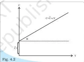
This is the geometry the entire chapter rests on. The line \(Y = a + bX\) (NCERT, p. 58) has two parts: \(a\), the intercept — the value of \(Y\) at \(X = 0\), where the line cuts the vertical axis.
And \(b\), the slope, drawn as \(\tan\theta\). Every graph that follows relabels this picture: the consumption function puts \(\bar{C}\) where \(a\) is, and \(c\) where \(b\) is.
Fig 4.2 — reading the consumption function
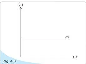
Here the intercept is \(\bar{C}\) — autonomous consumption, the spending that happens at zero income — and the slope is \(c = \tan\alpha\), the MPC (NCERT, p. 58). Reading the graph: the higher the line starts, the bigger the autonomous consumption; the steeper the line, the bigger the MPC.
Fig 4.3 — why the investment line is horizontal
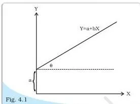
Investment is the one component that does not slope upward. The horizontal line at height \(\bar{I}\) (NCERT, p. 58) says plainly: planned investment stays \(\bar{I}\) whether income is 100 or 1,000. Contrast this with the consumption line — that is the whole difference between the two components.
Fig 4.4 — aggregate demand by vertical addition
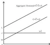
To get aggregate demand, add consumption and investment vertically at every income level: \(OL = \bar{C} + \bar{I}\) is the new intercept, and the slope stays \(c\) (NCERT, p. 59). Because \(\bar{I}\) is the same at every income, the AD line is the consumption line lifted up, still parallel to it.
The caption carries the chapter’s core idea: this line shows planned demand — ex ante, not actual.
Fig 4.5 — the 45 degree line as aggregate supply
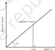
The 45-degree line is aggregate supply at fixed prices (NCERT, p. 59). Every point on it has the same horizontal and vertical coordinates, so it maps any GDP on the horizontal axis to exactly that much supply on the vertical axis.
The book’s own move: at GDP 1,000, supply is 1,000, shown where the vertical line from the GDP axis meets the 45-degree line. So supply never blocks demand — with unused resources, any demanded output arrives at the same price. On multiplier diagrams, use the 45-degree line as a measuring rod: horizontal gains equal vertical gains.
Fig 4.7 — the multiplier gap when AD shifts
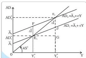
This is the picture of the multiplier (NCERT, p. 61). A rise of \(\Delta\bar{I}\) lifts the AD line from \(AD_1\) to \(AD_2\), parallel to itself. At the old income \(Y_1^*\), demand now exceeds output by the vertical gap \(E_1F\).
That gap is excess demand, and it measures only the first injection. The new equilibrium settles at \(E_2\), where the shifted AD line cuts the 45-degree line. The horizontal distance \(E_1G\) is the total gain in output — bigger than \(E_1F\), because the first injection is re-spent round after round.
That is the multiplier in one picture: a small vertical gap, a long horizontal gain.
Fig 4.6 and Fig 4.8 complete the set but appear only in the book. Fig 4.6 is the equilibrium diagram itself: the AD line and the 45-degree line drawn together, crossing at point E, with equilibrium income \(OY_1\) read off the horizontal axis (NCERT, p. 59–60).
Fig 4.8 shows the Paradox of Thrift: when the MPC falls, the AD line swings down — its slope gets flatter around the same intercept — and income contracts (NCERT, p. 63).
Definitions: the terms the chapter wants you to know
Quick-reference glossary for definition questions and distinctions. Page numbers send you to where each term is built.
| Term | Plain meaning | NCERT page |
|---|---|---|
| Ex ante | Planned, intended values of consumption, investment or output before the period runs | p. 54 |
| Ex post | Actual, accounting values as measured after the period | p. 54 |
| Autonomous consumption | Consumption that would occur even at zero income, \(\bar{C}\) | p. 54 |
| Induced consumption | Consumption that responds to income, \(cY\) | p. 54 |
| MPC | Change in consumption per unit change in income, \(\Delta C/\Delta Y\) | p. 55 |
| MPS | Change in saving per unit change in income, \(1 – MPC\) | p. 55 |
| APC | Consumption per unit of income, \(C/Y\) | p. 55 |
| APS | Saving per unit of income, \(S/Y\) | p. 55 |
| Autonomous investment | Planned investment treated as given, \(\bar{I}\), independent of income | p. 56 |
| Aggregate demand | Total planned spending on final goods at each income level | p. 56 |
| Equilibrium | The income level where planned output equals planned demand, \(Y = AD\) | p. 57, 60 |
| Parametric shift | A shift or swing of a line caused by a change in a parameter | p. 65 |
| Effective demand | The principle that, with fixed prices, output is determined solely by aggregate demand | p. 65 |
| Autonomous expenditure multiplier | Ratio of the total gain in output to the autonomous change that caused it, \(1/(1-c)\) | p. 62, 65 |
| Paradox of thrift | Economy-wide attempts to save more leave total saving unchanged or lower | p. 62–64 |
| Full employment | Income level at which all factors of production are fully employed | p. 64 |
| Deficient demand | Equilibrium output below full-employment output; prices tend to fall in the long run | p. 64 |
| Excess demand | Equilibrium output above full-employment output; prices tend to rise in the long run | p. 64 |
Formulas: the equations that do the work
Every numbered equation of the chapter, with each symbol named. Units: income, consumption, saving and investment are all in rupees — crores of rupees in the book’s exercise 5.
| Equation | What the symbols mean | NCERT page |
|---|---|---|
| \(C = \bar{C} + cY\) (4.1) | Consumption = autonomous consumption \(\bar{C}\) + induced consumption \(cY\); \(c\) is the MPC | p. 54 |
| \(MPC = \Delta C/\Delta Y = c\) | Extra consumption per extra rupee of income; a number between 0 and 1 | p. 54 |
| \(S = Y – C\), \(MPS = 1 – c\) | Saving is unconsumed income; \(\Delta S/\Delta Y = s = 1 – c\), so \(c + s = 1\) | p. 55 |
| \(APC = C/Y\), \(APS = S/Y\) | Average consumption and average saving per unit of income | p. 55 |
| \(I = \bar{I}\) (4.2) | Planned investment is a given constant, autonomous of income | p. 56 |
| \(AD = \bar{C} + \bar{I} + cY\) | Two-sector aggregate demand at each income; in equilibrium the book writes it as \(Y = \bar{A} + cY\) (4.3) | p. 56 |
| \(Y = (\bar{C} + \bar{I})/(1 – c)\) (4.4) | Equilibrium income in the two-sector model; also written \(Y = \bar{A}/(1-c)\) | p. 60 |
| \(\Delta Y/\Delta \bar{A} = 1/(1 – c) = 1/\text{MPS}\) (4.5) | Investment (autonomous expenditure) multiplier — a pure number; rises with \(c\), falls with \(s\) | p. 62 |
Where students slip in this chapter
These are the confusions the chapter itself warns about — each one is in the text before it shows up in your answer script.
| Mistake | Correct rule | How to check your answer |
|---|---|---|
| Treating planned and actual values as the same thing | Ex ante means planned, ex post means actual; the gap between them lands in unintended inventory change (NCERT, p. 54, 56–57) | Ask: would this equality still hold if plans went wrong? Inventories are the balancing item. |
| Reading \(Y = \bar{A} + cY\) as the Chapter 2 accounting identity | It holds only in equilibrium; outside equilibrium, stocks pile up or run down (NCERT, p. 56–57) | Pick an income above equilibrium, compute AD, and watch the gap appear. |
| Applying the multiplier to total income | The multiplier applies only to a change in autonomous expenditure, \(\Delta\bar{A}\) (NCERT, p. 62) | Name what changed (\(\Delta\bar{I}\) or \(\Delta\bar{C}\)) and multiply only that amount. |
| Believing a higher MPS raises the multiplier | It lowers it: the multiplier is \(1/\text{MPS}\), so a bigger MPS shrinks it (NCERT, p. 62) | Try MPS = 0.5 (multiplier 2) against MPS = 0.2 (multiplier 5). |
| Confusing a shift with a swing | A change in \(\bar{A}\) shifts the AD line in parallel; a change in MPC/MPS swings it (NCERT, p. 63) | Which parameter changed? Intercept change → shift; slope change → swing. |
| Expecting thrift to raise total saving | The Paradox of Thrift: income falls and total saving stays the same or falls (NCERT, p. 62–64) | Recompute \(S = Y – C\) at the new equilibrium income, not the old one. |
How this chapter is tested and how to answer
No marks figures are promised here — what is reliable is the match between the closing exercises and the ideas above. The exercises at the end of the chapter (NCERT, p. 65) revisit the model section by section:
- Exercise 1 asks for the meaning of the MPC and its relation to the MPS. A full answer gives \(MPC = \Delta C/\Delta Y\), then derives \(s = 1 – c\) from \(S = Y – C\) (NCERT, p. 54–55).
- Exercise 2 asks for the difference between ex ante and ex post investment — planned versus actual, with the inventory example (NCERT, p. 54).
- Exercise 3 asks about a parametric shift: when the slope falls, the line swings down; when the intercept rises, it shifts up, parallel (NCERT, p. 63).
- Exercise 4 asks for effective demand and for deriving the multiplier — start from \(Y = \bar{A} + cY\), solve for \(Y\), and show \(1/(1-c)\) (NCERT, p. 62, 65).
- Exercise 5 is the numerical: it gives autonomous expenditure, the MPS and an income level, and asks whether the economy is in equilibrium (NCERT, p. 56, 60).
- The closing exercise asks for the Paradox of Thrift — the swing of the AD line and why saving does not increase (NCERT, p. 62–64).
For the equilibrium-check type of numerical (Exercise 5), use this method every time:
- Turn the MPS into the MPC: \(c = 1 – \text{MPS}\).
- Write the aggregate demand equation with the given values: \(AD = \bar{A} + cY\).
- Compute AD at the stated income and compare with \(Y\): equality means equilibrium; \(AD \gt Y\) means excess demand (planned demand exceeds output); \(AD \lt Y\) means excess supply (output exceeds planned demand, so inventories accumulate).
Worked check with \(C = 60 + 0.75Y\), \(\bar{I} = 40\) (equilibrium at \(Y = 400\), as shown above). At \(Y = 420\): \(AD = 100 + 0.75(420) = 415 \lt 420\), not equilibrium — excess supply. At \(Y = 380\): \(AD = 100 + 285 = 385 \gt 380\), excess demand. Only at \(Y = 400\) do the plans match.
One honest reminder: textbook contents and the examinable syllabus are not always identical — check the current official syllabus.
Revision summary: the chapter in ten lines
Built from the chapter’s own Summary on page 65, in plainer words for the night before:
- The model fixes the final goods price and the interest rate; with unused resources, aggregate supply is perfectly elastic — price plays no role in output.
- Under the effective demand principle, output is determined solely by aggregate demand.
- Two-sector demand is \(AD = \bar{C} + \bar{I} + cY\); equilibrium is where planned output equals it, \(Y = AD\).
- Algebraically, equilibrium income is \((\bar{C} + \bar{I})/(1 – c)\).
- The multiplier is \(1/(1-c) = 1/\text{MPS}\): a change in autonomous spending changes income by more than itself.
- A change in \(\bar{A}\) shifts the AD line; a change in MPC/MPS swings it.
- The Paradox of Thrift: more saving reduces income, and total saving stays the same or falls.
- Equilibrium income need not be the full-employment income.
- Deficient demand (output below full employment) pushes prices down in the long run; excess demand pushes them up.
Now the Key Concepts (NCERT, p. 65) as a self-test — cover the list and say one correct sentence about each:
- Aggregate demand — total planned spending on final goods at each income.
- Aggregate supply — planned output of final goods; at fixed prices it is perfectly elastic.
- Ex ante / ex post — planned versus actual values.
- Ex ante consumption / ex ante investment — the two planned components that make up AD.
- Unintended changes in inventories — the unsold stock that appears when planned demand falls short.
- Marginal propensity to consume — extra consumption per extra unit of income.
- Autonomous change — a spending change that comes from outside the model, not from income.
- Parametric shift — a shift or swing of a line caused by a parameter change.
- Effective demand principle — output follows demand at fixed prices.
- Autonomous expenditure multiplier — the output gain per rupee of autonomous spending.
- Paradox of thrift — universal thrift leaves saving unchanged or lower.
- Equilibrium — planned demand equals planned output.
Related resources and sources
This chapter sits in the middle of Class 12 macroeconomics. The chapter after it, Government Budget and the Economy, extends the same model with taxes and government spending. For the rest of the course, use the Class 12 Economics notes, the Class 12 revision notes hub or the main CBSE notes index.
If you are also revising the micro half of the year, the Production and Costs notes are the matching resource.
The official Introductory Macroeconomics textbook page on ncert.nic.in hosts the full book as free PDFs — the same source as the download card above.
This page describes the NCERT Reprint 2026-27 edition of Introductory Macroeconomics as published on the official NCERT site. NCERT settles the textbook, its edition and its PDFs; CBSE settles the examinable syllabus. Since textbook contents and the examinable syllabus are not always identical, check the current official syllabus before deciding what to study.
Reference: NCERT Class 12 Introductory Macroeconomics textbook, chapter 4, official edition on ncert.nic.in.
Frequently asked questions
What is the investment multiplier formula in class 12 macroeconomics?
The investment multiplier is \(\Delta Y/\Delta \bar{A} = 1/(1 – c) = 1/\text{MPS}\) (NCERT, p. 62). It gives the total increase in income from a one-rupee rise in autonomous spending. With MPC 0.75, the multiplier is \(1/0.25 = 4\).
Why is the aggregate supply curve drawn as a 45 degree line?
With the price level fixed and unused resources available, whatever level of GDP is demanded can be supplied at the same price. Every point on a \(45^\circ\) line has equal horizontal and vertical coordinates, so it maps any GDP to exactly that much supply (NCERT, p. 59).
What is the difference between ex ante and ex post investment?
Ex ante investment is planned; ex post investment is what actually happens (NCERT, p. 54). If a shopkeeper plans to add ₹40,000 to stock but an unexpected sales surge of ₹15,000 is met from stock, actual inventory investment is only ₹25,000. The difference shows up as an unintended inventory change.
Why does the paradox of thrift say that more saving leaves total saving unchanged?
When everyone raises the MPS, the MPC falls and the AD line swings down. Income contracts, and at the new lower income the saving per unit is higher but the income itself is smaller — the two effects cancel, so total planned saving stays the same or falls (NCERT, p. 62–64).
How do you calculate equilibrium income when consumption and investment are given?
Add the autonomous parts and divide by \(1 – c\): \(Y = (\bar{C} + \bar{I})/(1 – c)\) (NCERT, p. 60). With \(C = 60 + 0.75Y\) and \(\bar{I} = 40\), \(Y = 100/0.25 = 400\).
What is the difference between autonomous consumption and induced consumption?
Autonomous consumption \(\bar{C}\) is the spending that happens even at zero income; induced consumption \(cY\) is the part that moves with income (NCERT, p. 54).
Explore Class 12 Economics Books
Related chapters: