
This page covers The Theory of the Firm under Perfect Competition, Chapter 4 of the NCERT Introductory Microeconomics textbook for Class 12 Economics. The chapter runs about 18 printed pages, and the official NCERT PDF of the chapter is available right here. The page is maintained for the current academic session using the NCERT information available to us.
Download the NCERT Class 12 Economics Chapter 4 PDF
If you want the chapter as it appears in the book — tables, diagrams, exercises and all — download The Theory of the Firm under Perfect Competition Class 12 NCERT PDF from the official NCERT website. It is the same file students and teachers use, and it opens directly without login.
Keep it beside this page: the explanations below follow the chapter section by section so you can match each idea to its place in the book.
| What the chapter holds | Count | Where it is used |
|---|---|---|
| Printed pages | 18 | |
| Sections in the chapter | 17 | |
| Figures with NCERT captions | 12 | |
| Tables | 8 | |
| Exercise questions | 27 | answered in our NCERT Solutions |
| Official NCERT PDF | Download the chapter PDF | the chapter exactly as NCERT publishes it |
Chapter 4 at a Glance
The table below lists what the chapter file actually holds — its sections, diagrams, tables and exercises — so you know the size of the chapter before you start.
| What is in the chapter | Count |
|---|---|
| Printed pages | 18 |
| Sections | 17 |
| Figures | 12 |
| Tables | 8 |
| Equations | 32 |
| Exercise questions | 27 |
What the Chapter Covers, Section by Section
This chapter answers one question: how does a profit-maximising firm in a perfectly competitive market decide how much to produce? The chapter’s own flow diagram below shows the route: it starts with the firm’s profit problem, derives the firm’s supply curve from it, and finally adds up all firms to get the market supply curve.

The chapter’s 17 sections fall into seven blocks:
- 4.1 Perfect Competition: Defining Features — the four features of a perfectly competitive market and what price-taking behaviour means.
- 4.2 Revenue — total revenue, average revenue, marginal revenue and the price line.
- 4.3 Profit Maximisation — the three conditions a firm’s output must satisfy to be profit-maximising.
- 4.4 Supply Curve of a Firm — how the short run and long run supply curves come from the cost curves.
- 4.5 Determinants of a Firm’s Supply Curve — technology, input prices and the unit tax.
- 4.6 Market Supply Curve — adding up individual firm supplies at every price.
- 4.7 Price Elasticity of Supply — measuring how strongly quantity supplied responds to price.
Key Concepts: Revenue, Profit Maximisation and Supply
A firm in perfect competition is a price-taker: it cannot choose its price, so its only real decision is how much to produce. The chapter finds that output by comparing revenue with cost. The chapter assumes the firm sells everything it produces, so ‘output’ and ‘quantity sold’ are used interchangeably (NCERT, p. 52).
Revenue: TR, AR and MR for a Price-Taking Firm
Because the price is fixed, every revenue idea in this chapter comes down to the market price \(p\). Three definitions do all the work (NCERT, p. 54):
- Total revenue \(TR = p \times q\) — the market price multiplied by the quantity sold.
- Average revenue \(AR = TR/q = p\) — total revenue per unit, which equals price.
- Marginal revenue \(MR = \Delta TR / \Delta q = p\) — the increase in total revenue from one more unit.
Why does \(MR\) equal price? If the firm sells one extra unit, that unit fetches exactly the market price. So total revenue rises by \(p\), and \(MR = p\). The same logic makes \(AR =\) price, and since \(TR = p \times q\) with \(p\) constant, the total revenue curve is an upward-sloping straight line through the origin with slope \(p\) (NCERT, p. 54).
Try it with an original example. A firm sells notebooks in a perfectly competitive market at Rs 25 per notebook.
| Output (q) | TR = 25 × q (Rs) | AR = TR/q (Rs) | MR = ΔTR/Δq (Rs) |
|---|---|---|---|
| 0 | 0 | — | — |
| 1 | 25 | 25 | 25 |
| 2 | 50 | 25 | 25 |
| 3 | 75 | 25 | 25 |
| 4 | 100 | 25 | 25 |
| 5 | 125 | 25 | 25 |
| 6 | 150 | 25 | 25 |
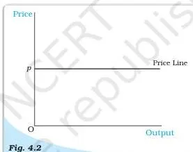
The price line at height \(p\) is also the demand curve facing the firm. It is perfectly elastic: at price \(p\) the firm can sell as much as it wants, and at any price above \(p\) it sells nothing (NCERT, p. 55). The total revenue curve is drawn and read in the diagram walkthrough below.
Profit Maximisation: The Three Conditions
Profit is the gap between what the firm earns and what it spends: \(\pi = TR – TC\) (NCERT, p. 56). The firm wants the output \(q_0\) where this gap is largest. Comparing revenue with cost gives the rule: keep producing as long as the next unit adds more to revenue than to cost, and stop where the two are equal.
That is condition 1, \(p = MC\).
Equality alone is not enough. For a positive output to be profit-maximising, three conditions must hold together (NCERT, p. 56):
- Price equals marginal cost: \(p = MC\), because for a price-taker \(MR = p\).
- Marginal cost is non-decreasing — it must not be falling at that output. If MC were falling, a slightly smaller output would give higher profit, so the point would not be a maximum.
- Price covers the relevant average cost: \(p \ge AVC\) in the short run, and \(p \ge AC\) in the long run. Otherwise the firm does better by producing nothing.
Here is a memory aid for the three conditions: “P-M-P”: Price equals MC, MC rising, Price covers average cost. Conditions 1 and 2 locate the output; condition 3 decides whether the firm produces at all.
The Firm’s Supply Curve, Shut Down and Break-Even
Once these conditions are in place, the firm’s supply curve follows directly. Since the firm produces where \(p = SMC\) on the rising part of the curve, the supply curve is a segment of the marginal cost curve — but only the part that satisfies condition 3. The two key conclusions (NCERT, pp. 59-60):
- Short run supply curve — the rising part of the SMC curve from the minimum AVC upwards, plus zero output for every price below minimum AVC.
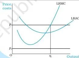
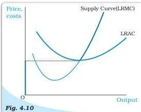
- Long run supply curve — the rising part of the LRMC curve from the minimum LRAC upwards, plus zero output for every price below minimum LRAC.
Two points on the cost curves matter for supply:
- The shut down point is the minimum AVC in the short run (where SMC cuts AVC) and the minimum LRAC in the long run. Below this price, production stops (NCERT, p. 61).
- The break-even point is the point of minimum average cost, where the firm earns only normal profit. Normal profit is the minimum profit needed to keep the firm in business, so it counts as part of total cost — an opportunity cost for the entrepreneur (NCERT, p. 61). Any profit above normal profit is super-normal profit.
| Short run | Long run | |
|---|---|---|
| Supply curve is | Rising part of SMC from minimum AVC upwards | Rising part of LRMC from minimum LRAC upwards |
| Shut down point | Minimum AVC (SMC cuts AVC) | Minimum LRAC |
| Break-even point | Minimum SAC | Minimum LRAC |
| If price is below the shut down point | Output is zero | Output is zero (firm exits) |
| Typical loss below break-even but above shut down | Firm produces despite a loss | Firm cannot stay in the market |
What Shifts a Firm’s Supply Curve
Because the supply curve is part of the marginal cost curve, anything that moves the MC curve moves supply. The chapter studies three shifters (NCERT, p. 62):
- Technological progress — an innovation lets the same inputs produce more output, lowering marginal cost at every level. The MC curve shifts right, so the supply curve shifts right: at any price, the firm supplies more.
- Higher input prices — if a factor such as labour becomes costlier, both average and marginal cost rise. The supply curve shifts left: at any price, the firm supplies less.
- A unit tax of Rs t — the firm pays an extra Rs t on every unit, so LRAC and LRMC both rise by Rs t. The long run supply curve shifts left.
Market Supply and Price Elasticity of Supply
An individual firm’s supply is only half the story; the market supply curve is what actually fixes the price. The rule is simple: at any price, add up what each firm supplies. This is horizontal summation — adding quantities, not prices (NCERT, p. 63).
Try a two-firm example. Firm 1 starts supplying once price reaches Rs 8, and firm 2 starts at Rs 12. Let the supply curves be \(S_1(p) = p – 8\) for \(p \ge 8\), and \(S_2(p) = 2(p – 12)\) for \(p \ge 12\). Then market supply is
- \(S_m(p) = 0\) for \(p \lt 8\);
- \(S_m(p) = p – 8\) for \(8 \le p \lt 12\) (only firm 1 produces);
- \(S_m(p) = (p – 8) + 2(p – 12) = 3p – 32\) for \(p \ge 12\) (both firms produce).
Check at \(p = 20\): firm 1 supplies 12 units, firm 2 supplies 16 units, and \(3(20) – 32 = 28\), which matches. If the number of firms in the market changes, the market supply curve shifts — more firms shift it right, fewer shift it left (NCERT, p. 63).
Price elasticity of supply measures how strongly quantity supplied responds to a price change (NCERT, p. 65):
\(e_s = \frac{\text{Percentage change in quantity supplied}}{\text{Percentage change in price}}\) For a vertical supply curve, quantity supplied does not respond to price at all, so \(e_s = 0\). For a positively sloped supply curve, a rise in price raises quantity supplied, so \(e_s \gt 0\). Like the price elasticity of demand, it is a unit-free number.
Formulas in Chapter 4 with a Worked Example
All the algebra in the chapter fits into five formulas. The table below states each one, what it means, and what the symbols stand for.
| Formula | Meaning | Symbols |
|---|---|---|
| \(TR = p \times q\) | Total revenue equals price times quantity sold | \(p\) = market price; \(q\) = output sold |
| \(AR = TR/q = p\) | Average revenue per unit equals the market price | \(TR\) = total revenue; \(q\) = output |
| \(MR = \Delta TR / \Delta q = p\) | Marginal revenue from one more unit equals the price | \(\Delta TR\) = change in total revenue; \(\Delta q\) = change in output |
| \(\pi = TR – TC\) | Profit is total revenue minus total cost | \(TC\) = total cost |
| \(e_s = \frac{\Delta Q}{Q} \times \frac{P}{\Delta P}\) | Price elasticity of supply | \(\Delta Q\) = change in quantity supplied; \(P\) = price |
Worked example: the price of a good rises from Rs 20 to Rs 30, and the quantity supplied rises from 500 to 700 units.
- Step 1: Percentage change in quantity supplied \( = \frac{700 – 500}{500} \times 100 = 40\%\).
- Step 2: Percentage change in price \( = \frac{30 – 20}{20} \times 100 = 50\%\).
\[ e_s = \frac{40}{50} = 0.8 \]
Final answer: \(e_s = 0.8\). Supply is relatively inelastic here because the percentage rise in quantity is smaller than the percentage rise in price.
How to Read the Diagrams in Chapter 4
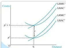
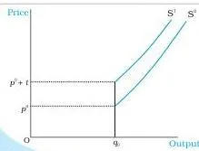
Every diagram in this chapter does one of two things: it compares a price with a cost curve, or it builds one curve from another. Keep that pattern in mind and the labels stop being scary.
The Total Revenue Curve: Slope Equals Price
Output is on the \(x\)-axis and revenue on the \(y\)-axis. The curve passes through the origin because zero output earns zero revenue. At output \(q_1\), the vertical height \(Aq_1\) is the total revenue, which equals \(p \times 1 = p\) for one unit; hence the slope of the line is \(Aq_1/Oq_1 = p\) (NCERT, p. 54).
That slope is the whole story of this chapter: every extra unit sold adds exactly the market price to total revenue.
Why the Falling Marginal Cost Intersection Is Wrong
The horizontal price line cuts the MC curve in two places: \(q_1\) where MC is falling, and \(q_4\) where MC is rising. At \(q_1\), every output level slightly to the left has price above MC, which means profit is higher at a smaller output — so \(q_1\) cannot be the profit-maximising output.
The valid intersection is on the rising part of MC, which is exactly condition 2 (NCERT, p. 56).
Price Below Average Cost: The Long Run Exit Case
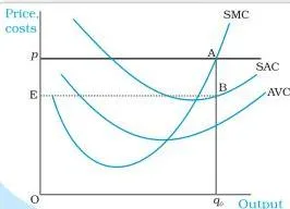
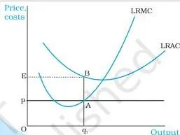
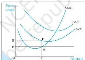
At output \(q_i\) the market price \(p\) lies below long run average cost. Total revenue is the rectangle \(OpAq_i\) while total cost is the larger rectangle \(OEBq_i\); the difference is the loss rectangle \(pEBA\).
In the long run the firm can avoid this entirely by exiting, since a shut down firm earns zero profit — which is better than a loss (NCERT, p. 58).
Building the Short Run Supply Curve
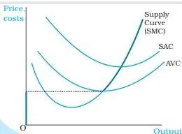
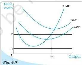
For a price \(p_1\) at or above minimum AVC, the firm equates \(p_1\) with SMC on the rising part and supplies \(q_1\). For a price \(p_2\) below minimum AVC, every positive output level has AVC above the price, so any output makes the firm lose more than shutting down; it supplies zero.
The bold part of the SMC curve from minimum AVC upwards, together with zero output below that price, is the short run supply curve (NCERT, p. 59).
Straight-Line Supply Curves and Price Elasticity
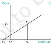
For a straight-line supply curve, elasticity at point \(S\) is the ratio \(Mq_0/Oq_0\), where \(M\) is where the extended supply line meets the quantity-axis. The position of \(M\) decides the value (NCERT, p. 66):
- \(M\) on the negative \(x\)-axis: \(Mq_0 \gt Oq_0\), so \(e_s \gt 1\).
- Supply line through the origin: \(M\) coincides with the origin, so \(e_s = 1\).
- \(M\) on the positive \(x\)-axis: \(Mq_0 \lt Oq_0\), so \(e_s \lt 1\).
The ratio, not the slope alone, decides elasticity.
Key Terms and Definitions in Chapter 4
These are the terms the chapter defines in bold. Check your understanding against the plain definitions below.
| Term | Plain definition |
|---|---|
| Perfect competition | A market with many buyers and sellers, a homogenous product, free entry and exit, and perfect information |
| Price-taking behaviour | A firm cannot sell anything above the market price, and can sell as much as it wants at the market price |
| Total revenue | Market price multiplied by the quantity sold: \(TR = p \times q\) |
| Average revenue | Total revenue per unit of output, equal to the price |
| Marginal revenue | The increase in total revenue from one extra unit of output, equal to the price |
| Price line | The horizontal line at height \(p\); the firm’s AR curve and its perfectly elastic demand curve |
| Profit | Total revenue minus total cost: \(\pi = TR – TC\) |
| Normal profit | The minimum profit needed to keep a firm in business; part of total cost, an opportunity cost for the entrepreneur |
| Super-normal profit | Profit earned over and above normal profit |
| Shut down point | Minimum AVC in the short run; minimum LRAC in the long run; below it the firm produces zero |
| Break-even point | Point of minimum average cost, where the firm earns only normal profit |
| Opportunity cost | The gain foregone from the second-best alternative activity |
| Unit tax | A tax imposed per unit of output sold, raising both LRAC and LRMC by the tax amount |
| Price elasticity of supply | The percentage change in quantity supplied divided by the percentage change in price |
Common Mistakes Students Make in This Chapter
Most errors in this chapter come from applying one rule where another belongs. Name the trap before you fall into it.
| Mistake | Correct rule | How to check your answer |
|---|---|---|
| Thinking a competitive firm can choose its price | The firm is a price-taker; it can only choose output, and must accept the market price | Ask: if this firm raised its price by one rupee, would it lose all buyers? If yes, it cannot set price |
| Accepting any \(MR = MC\) point as profit-maximising | MC must be non-decreasing at that output; the falling MC intersection gives lower profit | Look at the MC curve: is it sloping up at your chosen output? If it slopes down, test a slightly smaller output |
| Producing when price is below minimum AVC | In the short run, price below minimum AVC means output is zero | Compare price with minimum AVC, not with average cost, in the short run |
| Treating normal profit as extra profit | Normal profit is part of total cost — the opportunity cost of staying in business | At the break-even point, profit is zero in the economic sense, yet the firm stays |
| Adding supply curves vertically | Market supply is the horizontal summation of firm supplies at each price | Pick a price, read each firm’s quantity, add the quantities — never add the prices |
Exam Notes: Turning the Chapter into Answers
The chapter ends with 27 exercise questions, and they map neatly onto its ideas. Practising by group makes revision faster.
| Questions | Ideas tested | What a full answer must do |
|---|---|---|
| Q1-6 | Market features, TR, price line, AR and MR | State the definition, then use the \(TR = p \times q\), \(AR = p\), \(MR = p\) reasoning |
| Q7-11 | Profit-maximising conditions, shutdown logic | Give all three conditions and explain each with the \(MR\) vs \(MC\) logic |
| Q12-18 | Short run and long run supply, shifts, elasticity | Quote the supply curve rule, then state the direction of shift (right or left) |
| Q19-27 | Numerical schedules, market supply tables, elasticity calculations | Show every column and every substitution; end with the unit |
For the numericals, set out the revenue or elasticity formula, substitute the given values line by line, and state the final number clearly. Note that textbook contents and the examinable syllabus are not always identical — check the current official syllabus for this session.
Quick Recap: The Main Takeaways of Chapter 4
- Firms in perfect competition are price-takers: they take the market price as given and choose only how much to supply.
- Total revenue is \(p \times q\), and for a price-taking firm, average revenue equals marginal revenue equals the market price.
- The firm’s demand curve is perfectly elastic — a horizontal line at the market price.
- The three profit-maximisation conditions: \(p = MC\); MC non-decreasing; and \(p \ge AVC\) in the short run or \(p \ge AC\) in the long run.
- The short run supply curve is the rising part of SMC from minimum AVC upwards, plus zero output below it; the long run supply curve is the same idea with LRMC and minimum LRAC.
- Technological progress shifts supply right; higher input prices and a unit tax shift it left.
- The market supply curve is the horizontal summation of individual firm supply curves.
- Price elasticity of supply is positive for positively sloped supply curves, zero for a vertical curve, and unit-free.
Related Class 12 Economics Chapters
- Chapter 3 Production and Costs — the chapter before this one, which builds the cost curves used here.
- Chapter 5 Market Equilibrium — the next chapter, where market supply meets market demand.
- All Class 12 subjects — the hub for every Class 12 chapter page.
- CBSE notes home — notes for all classes and subjects.
Sources and data verification
This listing is maintained for the 2026-27 academic session using the NCERT textbook information available to us. NCERT remains the authority for confirming the latest edition.
- The figures in this page describe NCERT Class 12 Economics — Introductory Microeconomics, Chapter 4: The Theory of the Firm under Perfect Competition, official NCERT edition. The official PDF is at ncert.nic.in.
- This page covers Chapter 4 only; other chapters of the book are covered on their own pages.
- This listing is maintained for the current academic session using the NCERT information available to us.
- NCERT settles textbook editions and PDFs; CBSE settles the curriculum, syllabus and examinations.
Reference: NCERT Class 12 Introductory Microeconomics textbook, chapter 4, official edition on ncert.nic.in.
Frequently Asked Questions on the Theory of the Firm under Perfect Competition
Why is the demand curve facing a perfectly competitive firm a horizontal line at the market price?
Because the firm is a price-taker. At the market price \(p\) it can sell as many units as it wants, and at any price above \(p\) it loses all its buyers, since every other firm sells the identical good and buyers know the market price. So the demand curve facing the firm is perfectly elastic at height \(p\).
Why must a profit-maximising firm produce where price equals marginal cost and marginal cost is rising?
If price exceeded marginal cost, the next unit would add more to revenue than to cost, so producing it would raise profit. If price were below marginal cost, the last unit would add more to cost than to revenue, so producing less would raise profit. Only \(p = MC\) stops the adjustment.
MC must not be falling there, because at a falling MC intersection, a slightly smaller output would already earn higher profit.
Why does a firm produce in the short run even when price is below average cost but above average variable cost?
Because the firm loses less by producing than by shutting down. Fixed costs must be paid whether output is zero or positive. As long as price covers average variable cost, producing contributes something toward fixed costs, so the loss is smaller than the loss of producing nothing.
What is the difference between the shut down point and the break-even point?
The shut down point is the minimum AVC in the short run (or minimum LRAC in the long run); below that price the firm produces zero output. The break-even point is the minimum AC, where the firm earns only normal profit. Between the two, the firm produces even though it makes a loss — until it reaches the shut down point.
How do you find price elasticity of supply using the geometric method?
For a straight-line supply curve, extend the line to the quantity-axis and call that point \(M\). Elasticity at a point \(S\) is the ratio \(Mq_0/Oq_0\). If \(M\) lies on the negative \(x\)-axis, \(e_s \gt 1\); if the line passes through the origin, \(e_s = 1\); if \(M\) lies on the positive \(x\)-axis, \(e_s \lt 1\).
Is normal profit really a cost for the firm?
Yes. Normal profit is the minimum profit required to keep the firm in its current business, and it is the opportunity cost of the entrepreneur’s time and money. Because it is a cost, it is included in total cost; profit above it is super-normal profit.
Explore Class 12 Economics Books
- Previous: Production and Costs
- Next: Government Budget and the Economy
Related chapters:
- Adam Smith
- A Simple Economy
- National Income Accounting