
These notes are the complete revision set for Chapter 4, Spatial Information Technology, from the NCERT Class 12 Geography Practical Work book (Part-II). Everything you need for last-minute revision is here — the definitions, the raster-versus-vector comparison, the five GIS components, the analysis operations and the exercise framework — compressed into tables and lists you can scan in minutes.
These notes follow the 2026-27 session and the rationalised NCERT edition. Page references such as (NCERT, p. 47) point back to the textbook so you can cross-check any point. For the full set of study material for this subject, see the Class 12 Geography notes hub.
Spatial Information Technology: What This Chapter Covers
The chapter opens with the questions spatial technology exists to answer: What is where? Why is it there? What will happen if it is shifted to a new location? Who benefits from the reallocation, and who loses?
Answering them needs more than a computer that can draw maps — it needs a system that combines data from many sources and supports a decision.
The concept chain the chapter builds runs like this (NCERT, p. 46-47):
- DBMS (Database Management System) — processes data using computer hardware and application software.
- Computer Assisted Cartography — prepares graphs, diagrams and maps with the same tools.
- Together they can process and display, but not answer “what if” questions.
- That gap is filled by the Spatial Information System, more commonly called the Geographical Information System (GIS).
After revising, you should be able to: define spatial data and Spatial Information Technology, name the five GIS components, contrast raster and vector formats with their trade-offs, and explain overlay and buffer analysis with an example each.
What Is Spatial Information Technology?
The word spatial comes from space. It refers to features and phenomena distributed over a geographically definable space, which means they have physically measurable dimensions (NCERT, p. 46). The chapter’s two everyday examples: the address of a municipal facility, and the boundaries of an agricultural holding.
Spatial Information Technology (SIT) is the use of technological inputs to collect, store, retrieve, display, manipulate, manage and analyse spatial information. It is an amalgamation of five technologies:
- Remote Sensing
- GPS (Global Positioning System)
- GIS (Geographical Information System)
- Digital Cartography
- Database Management Systems
What Is GIS? The System Behind the Technology
Since the mid-1970s, advanced computing systems have been able to process georeferenced information: organise spatial and attribute data, integrate them, locate specific records, execute computations and analysis, and evolve a decision support system. A system capable of all this is a Geographical Information System (NCERT, p. 47).
The chapter’s definition in plain words: GIS is a system for capturing, storing, checking, integrating, manipulating, analysing and displaying data that are spatially referenced to the Earth. It normally involves a spatially referenced computer database and appropriate applications software.
Two points lift GIS above a mere map-making tool:
- It is an amalgamation of Computer Assisted Cartography and DBMS — it can draw and analyse.
- It draws conceptual and methodological strength from both spatial and allied sciences: Computer Science, Statistics, Cartography, Remote Sensing, Database Technology, Geography, Geology, Hydrology, Agriculture, Resource Management, Environmental Science and Public Administration.
The phrase to remember: GIS is a decision support system. That is what separates it from plain mapping and data processing.
Spatial Data vs Non-Spatial (Attribute) Data
Geographical information comes in two types. Spatial data are characterised by three forms of appearance — positional, linear and areal. Non-spatial (attribute) data describe the spatial data (NCERT, p. 47).
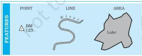
The figure above shows the three forms a feature can take on a map: a point (a single location), a line (a sequence of points, e.g. a road) and an area (an enclosed region, e.g. a district).
These forms must be geometrically registered to a generally accepted coordinate system and coded so they can be stored in the GIS database.
The chapter’s Box 4.1 contrasts the two data types with a pair of tables (NCERT, p. 47):
- Stock register of a cycle shop — part number, quantity, description (wheel spoke, ball bearing, wheel rim, tyre). This is non-spatial: the parts could be located anywhere; their position on a map is irrelevant.
- Literate population in states, 1981 — state, % male, % female. This is spatial: each state name has a definite location on a map, so the record can be used in GIS.
Building the spatial database. The chapter calls spatial data the most important prerequisite of a spatial or geographical information system. In a GIS core it can be built in three ways (NCERT, p. 48):
- Acquire data in digital form from a data supplier.
- Digitise existing analogue data.
- Carry out one’s own surveys of geographic entities.
The choice of source is governed by three factors: the application area itself, the available budget, and the type of data structure (vector or raster). Most users take spatial data from topographical or thematic maps, in hard copy or digital form. All such maps share three characteristics (NCERT, p. 48):
- A definite scale relating the map to the surface it represents.
- Symbols and colours that define the attributes of mapped entities.
- An agreed coordinate system that fixes the location of entities on the Earth’s surface.
The Five Components of GIS
The five components are Hardware, Software, Data, People and Procedures (NCERT, p. 49). Fig. 4.2 shows them working as a single system.
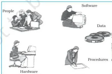
- Hardware — the processing, storage, display, and input and output sub-systems (computer, screen, digitiser, scanner, plotter).
- Software — modules for data entry and editing; analysis, transformation and manipulation; and data display and output.
- Data — spatial data plus related tabular data; the chapter calls this the backbone of GIS. The digital map is the basic data input, and tabular data about map objects can be attached.
- People — users from hardware and software engineers to resource and environmental scientists, policy-makers, and monitoring and implementing agencies.
- Procedures — how data are retrieved, input, stored, managed, transformed, analysed and finally presented.
Memory device: H-S-D-P-P → “Hard-working Students Do Perfect Projects.” Hardware, Software, Data, People, Procedures. Cover the list and recall the five before reading on — this is the most direct five-item list in the chapter.
Spatial Data Formats: Raster and Vector
Spatial data are represented in two formats: raster and vector (NCERT, p. 50).
Take the chapter’s example — a line drawn diagonally on a piece of paper. Raster subdivides the paper into a matrix of small rectangles (cells), like a sheet of graph paper.
Each cell is assigned a position in the data file and a value based on the attribute at that position; any individual pixel is identified by its row and column coordinates (Fig. 4.3). Vector records the line by simply recording the coordinates of its starting and ending points.
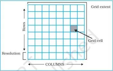
Raster resolution. The relationship between cell size and the number of cells is the resolution of the raster (NCERT, p. 50). Fig. 4.4 shows the effect of grid size:
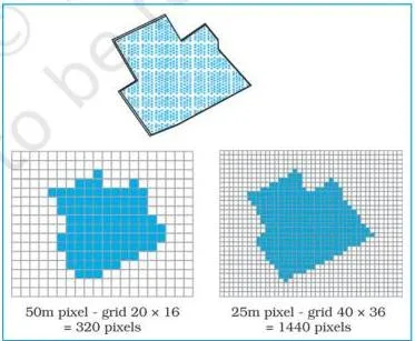
Large cells give fewer cells and coarser detail; small cells give finer detail but much larger files. The same feature can be blocky at one grid size and recognisable at a finer one.
Vector coordinates. A vector point is expressed as two or three numbers — X, Y in 2D, or X, Y, Z in 3D (NCERT, p. 51). X is the distance from the left side of the paper, Y the distance from the bottom, and Z the point’s elevation above or below the paper. Fig. 4.5 shows the model:
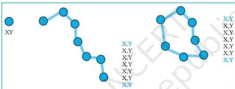
In a vector model, lines and areas are built from sequences of points stored by their real (earth) coordinates. Lines have a direction given by the ordering of points; polygons can be built from points or lines; and vectors can store information about topology, the spatial relationships between features. Manual digitising is the best way of vector data input.
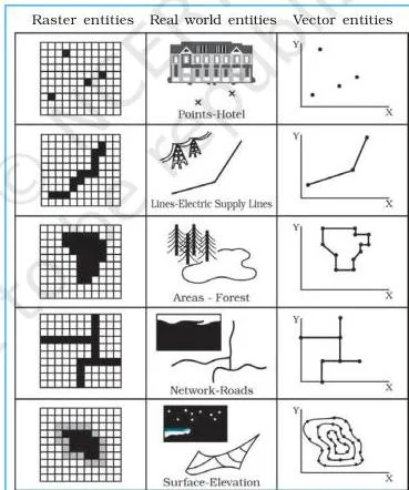
Fig. 4.6 places the two formats side by side: the same entities appear as blocky cells in raster and as crisp lines and outlines in vector.
Analogy to keep them apart: raster is a mosaic of tiles — every tile has one colour and the picture is built from thousands of them; vector is a connect-the-dots drawing — only the key points are recorded and lines join them.
When each format is used (NCERT, p. 51):
- Raster files — digital representations of aerial photographs, satellite images and scanned paper maps; when costs must be kept down; when the map does not require analysis of individual features; when “backdrop” maps are required.
- Vector files — highly precise applications; when file sizes matter; when individual map features require analysis; when descriptive information must be stored.
The complete trade-off is in Box 4.2 (NCERT, p. 52):
| Raster model | Vector model |
|---|---|
| Advantages: simple data structure; easy and efficient overlaying; compatible with satellite imagery; high spatial variability efficiently represented; simple for own programming; same grid cells for several attributes | Advantages: compact data structure; efficient for network analysis; efficient projection transformation; accurate map output |
| Disadvantages: inefficient use of computer storage; errors in perimeter and shape; difficult network analysis; inefficient projection transformations; loss of information when using large cells; less accurate maps | Disadvantages: complex data structure; difficult overlay operations; high spatial variability inefficiently represented; not compatible with satellite imagery |
Where the Numbers Are: Resolution and Coordinates
This chapter has no formulas — do not hunt for any. The only quantitative ideas are:
- Raster resolution: the inverse relationship between cell size and cell count — smaller cells mean higher resolution but larger storage.
- Vector coordinates: the X, Y, Z values that fix a point’s position and elevation.
Treat both as concepts with examples, not as calculation work.
Sequence of GIS Activities: How Data Gets In
The GIS work sequence has five steps (NCERT, p. 53). This exact order is worth memorising — the textbook’s 125-word exercise asks for it:
- Spatial data input
- Entering the attribute data
- Data verification and editing
- Spatial and attribute data linkage
- Spatial analysis
Route 1: acquiring digital data sets from a supplier. Suppliers make digital data available from small-scale maps to large-scale plans, saving users the overhead of digitising or collecting their own data. But serious attention must go to data compatibility: projection, scale, base level and attribute descriptions can differ between sources.
At a practical level, users must check (NCERT, p. 53): the scale of the data; the geo-referencing system used; the data collection techniques and sampling strategy; the quality of data; the classification and interpolation methods; the size and shape of individual mapping units; and the length of record. Integration problems are especially common when compiling inter-province or inter-district data sets.
Route 2: creating digital data by manual input. Four stages: entering spatial data, entering attribute data, verification and editing, and linking spatial to attribute data (NCERT, p. 53). The two common ways of inputting spatial data are digitising and scanning.
Scanners and CCDs. Scanners convert analogue data into digital grid-based images — a line map becomes a high-resolution raster image, usable directly or processed further to get vector topology. There are two basic types: those that record data step by step, and those that scan a whole document in one operation.
The scanner’s camera carries special sensors called Charged Coupled Devices (CCDs) — semi-conductor devices arranged in an array that translate the photons of light falling on their surface into counts of electrons, recorded as a digital value (NCERT, p. 54). A scanned image always carries the smudges and defects of the original, so excess data must be removed before use.
Entering attribute data. Attribute data define the properties of a spatial entity that are not spatial — for a road: width, surface type, estimated traffic, specific traffic regulations (NCERT, p. 54-55). They can be keyed in manually or imported from published records, official censuses, primary surveys or spreadsheets using a standard transfer format.
Data Verification, Editing and Conversion
Captured spatial data must be verified for errors. The classic check: produce a computer plot of the data, preferably on a translucent sheet at the same scale as the original, lay it over the original on a light table, and compare visually, working systematically from left to right and top to bottom, marking missing data and locational errors (NCERT, p. 55).
Errors fall into three groups:
| Error type | Cause |
|---|---|
| Spatial data incomplete or double | Omissions in manual input of points, lines or polygons; in scanned data, gaps between lines where raster-vector conversion failed to join up all parts of a line |
| Spatial data at the wrong scale | Digitising at the wrong scale; in scanned data, incorrect geo-referencing values |
| Spatial data distorted | Base maps not scale-correct; aerial photo lens distortion, relief and tilt displacements; paper maps damaged by rain, sunshine or frequent folding |
Correction tools: move entities with the screen cursor; use keyboard commands to move, rotate, erase, insert, stretch or truncate entities; remove excess coordinates with weeding algorithms; change faulty raster cell values. Topology of vector line and polygon networks is generated only after spatial errors are corrected (NCERT, p. 55-56).
Conversion rule: all layers used together must be in one format — all vector or all raster. Because most analysis is done in the raster domain, conversion usually runs vector to raster by overlaying a grid of user-defined cell size. Raster to vector conversion is done mainly for data reduction, since raster storage is much larger (NCERT, p. 56).
Linking Spatial and Attribute Data: Exact, Hierarchical and Fuzzy Matching
Linkages must be undertaken carefully: linking attribute data to a non-related spatial layer leads to chaos in analysis, and matching one data layer with another is equally significant (NCERT, p. 56).
Example: to find the mortality rate from malnutrition among children under 10 in a state, one file holds the number of children in that age group and another holds the mortality from malnutrition. Link the two files, then divide one figure by the other to get the rate.
The two named matching modes (NCERT, p. 56-57):
| Mode | How it works | Chapter’s example |
|---|---|---|
| Exact matching | A key common to both files (e.g. town names) is used to extract and join matching records into a new file | Information about towns in two files joined by town name |
| Hierarchical matching | Data for small areas are added together until the grouped areas match the larger areas, then matched exactly | Frequent large-area land use data matched with less frequent small-area land transformation data |
| Fuzzy matching | Boundaries never align; the two sets are overlaid and the combinations are computed | Crop field edges vs soil-type boundaries — overlay to find the most productive soil for a crop |
One condition governs all three: spatial data sets link only when they relate to the same geographical area (NCERT, p. 57).
Spatial Analysis: Overlay and Buffer Operations
The strength of GIS lies in its analytical capabilities. The chapter names four spatial analysis operations but details only two (NCERT, p. 57):
- Overlay analysis
- Buffer analysis
- Network analysis
- Digital Terrain Model
Overlay analysis
Overlay is the hallmark of GIS: two or more thematic layers of maps of the same area are integrated to obtain a new map layer (NCERT, p. 57). It works like sieve mapping — laying tracings of maps on a light table to make comparisons and obtain an output map (NCERT, p. 59).
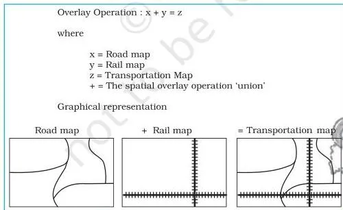
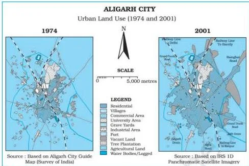
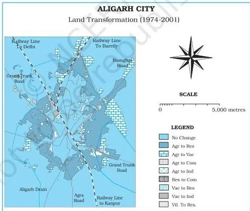
Application 1 — land transformation. Overlay studies changes in land use and land cover over two periods. The chapter’s case: Aligarh city, Uttar Pradesh. Fig. 4.8 shows urban land use in 1974 and in 2001; overlaying the two maps yields the land transformation map of Fig. 4.9, and the urban sprawl over the period is mapped (NCERT, p. 58-59).
Application 2 — suitability analysis. Overlay also tests a proposed land use against the existing conditions of an area.
Buffer analysis
A buffer of a specified distance can be created along any point, line or area feature (NCERT, p. 59). It locates the areas or populations benefited or denied facilities and services — hospitals, medical stores, post offices, asphalt roads, regional parks — and can study the impact of point sources of air, noise or water pollution on human health.
This kind of analysis is called proximity analysis.
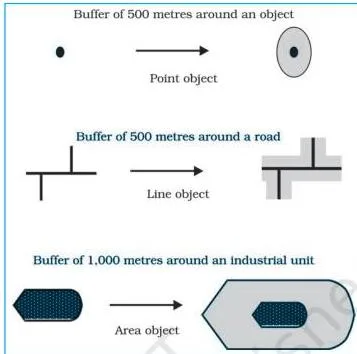
Chapter example: the number of households living within a one-kilometre buffer from a chemical industrial unit are the ones affected by the industrial waste discharged from the unit.
Hospital case study. Using ArcView/ArcGIS, Geomedia or the free QGIS software, buffers of 2, 4, 6, 8 and 10 kilometres were created around cities with major hospitals — Saharanpur, Muzaffarnagar, Meerut, Ghaziabad, Gautam Budh Nagar and Aligarh (NCERT, p. 59-60).
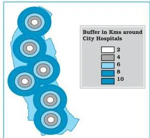
Reading the result: areas closer to the cities are better served; people living farther away travel long distances to use medical services, and their areas are the least benefitted. The chapter’s internet sources for exploring spatial data on your own include ISRO’s Bhuvan geoportal (NCERT, p. 60).
Key Terms: Definitions and Examples at a Glance
One table, every examinable term. Meanings are in plain words; examples are the chapter’s own.
| Term | Meaning | Example |
|---|---|---|
| Spatial data | Data about features with positional, linear or areal form in a geographically definable space | Literate population by state — state names have fixed map locations |
| Non-spatial (attribute) data | Data that describe spatial features but carry no location of their own | Cycle shop stock register — parts could be stored anywhere |
| Spatial Information Technology | Technological inputs for collecting, storing, retrieving, displaying, manipulating, managing and analysing spatial information | Amalgamation of Remote Sensing, GPS, GIS, Digital Cartography and DBMS |
| GIS | System for capturing, storing, checking, integrating, manipulating, analysing and displaying data spatially referenced to the Earth | Overlay of Aligarh land-use maps to map urban sprawl |
| DBMS | Computer-based data processing using hardware and application software | Processing the cycle shop stock register |
| Computer Assisted Cartography | Preparing maps and diagrams using computer hardware and software | Map output in any GIS software |
| Raster data | Features represented as a matrix of grid cells, each with a position and a value | Satellite image, scanned paper map |
| Resolution | The relationship between cell size and the number of cells in a raster | Smaller cells → finer detail but larger files |
| Vector data | Features stored as points with coordinates; lines and polygons built from ordered points | Digitised road network |
| Topology | Spatial relationships between features, storable in vector format | Which polygons share a boundary |
| Digitising | Manual input of spatial data using a digitiser | Digitising a paper map into vector layers |
| Scanning | Converting analogue data into digital grid-based images | Line map → high-resolution raster image |
| CCD | Semi-conductor sensor that translates light photons into electron counts recorded as digital values | Sensors in a scanner’s digital camera array |
| Overlay | Integrating two or more thematic layers of the same area into a new map layer | Aligarh 1974 + 2001 land use → transformation map |
| Buffer | A zone of specified distance around a point, line or area feature | 1 km zone around a chemical industrial unit |
| Proximity analysis | Analysis using buffers to locate areas or populations served or affected by features | Households within 1 km of a chemical unit affected by its waste |
| Exact matching | Joining records from two files using a key common to both | Two town files joined by town name |
| Hierarchical matching | Aggregating small-area data until grouped areas match larger areas | Land use + land transformation data matched by aggregation |
| Overlay of unmatched boundaries | Overlaying data sets whose boundaries never align and computing combinations | Crop field edges vs soil-type boundaries |
| Under/over shoots | Digitising errors where a line stops short of or overshoots its junction | Scanned-data gaps, not under/over shoots |
| Weeding | Removing excess coordinates that define a line | Cleaning a digitised line to its essential points |
Worked Examples: Overlay and Buffer with Fresh Numbers
Two original problems that rehearse the chapter’s two analysis methods. Try them yourself before reading the steps.
Worked Example 1: Overlay change detection (method: overlay analysis)
A municipal area covers 50 \( \text{km}^2 \). Urban area in 1971: 8 \( \text{km}^2 \). Urban area in 2021: 17 \( \text{km}^2 \). Of the 2021 urban area, 6 \( \text{km}^2 \) was already urban in 1971.
Step 1: Find the new urban expansion — the 2021 urban area that was not urban in 1971:
\[ \text{New expansion} = 17\ \text{km}^2 – 6\ \text{km}^2 = 11\ \text{km}^2 \]
Step 2: Find the net change in urban area between the two dates:
\[ \text{Net change} = 17\ \text{km}^2 – 8\ \text{km}^2 = 9\ \text{km}^2 \]
Step 3: Interpret the difference.
The overlay-derived expansion (11 \( \text{km}^2 \)) is larger than the net change (9 \( \text{km}^2 \)) because \( 8 – 6 = 2\ \text{km}^2 \) of the 1971 urban area was converted to other uses by 2021.
Net change hides this internal turnover; overlay reveals it.
Conclusion: new urban expansion 11 \( \text{km}^2 \); net change 9 \( \text{km}^2 \); overlay detects both growth and conversion, which a simple difference misses.
Worked Example 2: Buffer ring interpretation (method: proximity analysis)
A proposed community health centre has buffer circles of 2 km and 5 km. The 2 km circle covers 12 villages; the 5 km circle covers 47 villages. Village cluster A lies 3.5 km from the centre.
Step 1: Locate cluster A.
At 3.5 km it falls between the two buffers — inside the 5 km circle but outside the 2 km circle.
Step 2: Find how many villages lie in the ring between 2 km and 5 km:
\[ \text{Ring villages} = 47 – 12 = 35\ \text{villages} \]
Step 3: Interpret access.
Households in the inner 2 km circle have the best access; the 35 villages in the ring have moderate access; villages beyond 5 km have the least benefit.
Conclusion: cluster A sits in the moderate-access ring holding 35 villages; buffer rings rank service access by distance from the facility.
Now reapply the same steps to the book’s hospital case: six cities, buffers of 2, 4, 6, 8 and 10 km, and the conclusion that areas closer to cities are better served.
Common Mistakes in Spatial Information Technology
Misconception autopsy: GPS vs GIS vs remote sensing. Students mix these three because all feed into spatial technology. Remote Sensing is how you acquire data — sensors on satellites or aircraft record the Earth from a distance. GPS is how you locate it — satellites give the exact coordinates of a point.
GIS is what you do with it — the system that captures, stores, analyses and displays spatially referenced data to support a decision. In the chapter’s chain, Remote Sensing and GPS are two of the five technologies amalgamated into Spatial Information Technology; GIS is the analytical heart of that amalgamation (NCERT, p. 46-47).
The confusions below are the ones most likely to trip up students in this chapter:
| Mistake | Correct rule | How to check your answer |
|---|---|---|
| “GIS = GPS” | GPS is a satellite-based positioning input that gives a point’s coordinates. GIS is the system that captures, stores and analyses spatially referenced data. | Ask: does the statement describe positioning or analysis? Positioning → GPS. |
| “Raster is better than vector” | Each format has defined strengths. Raster suits satellite imagery, cheap storage and simple overlay; vector is compact, precise, good for network analysis and stores topology. | Match the format to the job: imagery → raster; precise individual features → vector. |
| “Overlay and buffer are the same” | Overlay combines thematic layers of the same area into a new layer. Buffer creates a distance zone around a feature for proximity analysis. | Overlay = layers stacked; buffer = rings around a feature. |
| “Attribute data are just tables and less important” | Attributes describe spatial features and must be linked carefully; linking them to a non-related spatial layer leads to chaos. | Does the data describe the feature? If yes, it must be linked correctly, not skipped. |
| “All analysis layers can be mixed freely” | All layers used together must share one format — all raster or all vector — so convert before analysis. | Check every layer’s format before overlaying. |
| “Verification is optional” | Unverified under/over shoots, scale errors and distortion corrupt results; editing often takes longer than input. | Do the light-table check on a translucent printout at the same scale. |
| “Spatial simply means has a location” | Spatial features sit in a geographically definable space with physically measurable dimensions. | Is the feature mappable with measurable extent? Then it is spatial. |
Exam Notes: Writing the Chapter’s Exercise Answers
These are frameworks — the points a complete answer must include — not model answers. The chapter’s exercises are on p. 61.
30-word questions (six of them). Each needs 2-4 precise points:
- Raster vs vector models: define each in one line (grid cells vs coordinates), give one contrast (storage or overlay ease), and one typical use of each.
- Overlay analysis: definition (integrating thematic layers of the same area into a new layer) plus one application (land-use change detection or suitability analysis).
- GIS over manual methods: the three map limitations (fixed presentation, predetermined themes, redrawing needed for any alteration) against the GIS advantages (interrogating displayed features, drawing maps from attribute queries, spatial operations on the integrated database, linking attribute items through shared location codes).
- Components of GIS: name all five — hardware, software, data, people, procedures.
- Ways to build spatial data in the GIS core: the three routes — digital supplier, digitising analogue data, one’s own surveys.
- Spatial Information Technology: definition (technological inputs to collect, store, retrieve, display, manipulate, manage and analyse spatial information) plus the five-part amalgamation.
125-word questions (two of them). Use a three-part paragraph plan:
- Raster and vector formats with an example: opening definition sentence; one paragraph on raster (grid cells, resolution, a satellite image example); one on vector (coordinate pairs, topology, a digitised map example); closing line on the Box 4.2 trade-off.
- Sequence of GIS activities: opening sentence naming the five steps; one line per step explaining what happens; closing line on why the sequence matters for data quality.
Multiple-choice set (Q1). Use elimination by concept:
- Spatial data forms — the three forms are positional, linear and areal; the complete option is the one listing all three.
- Analysis module — of storage, display, output and buffering, only buffering is an analysis operation requiring the analysis module software.
- Raster disadvantage — of the four options, only “difficult network analysis” is a raster disadvantage from Box 4.2; the others are raster advantages.
- Vector advantage — of the four options, only “compact data structure” is a vector advantage; the rest are vector disadvantages.
- Urban change detection — overlaying two time-period layers is an overlay operation.
Wherever a definition is needed, attach the chapter’s own case study — Aligarh for overlay, the hospital buffers for proximity analysis — to show the concept in use. The official NCERT textbook portal has the full chapter if you need to verify any page reference.
Revision Recap: The Chapter on One Page
- The chain: DBMS + Computer Assisted Cartography → processing and display only → Spatial Information System → GIS (p. 46-47).
- Spatial: features in a geographically definable space with measurable dimensions. SIT = the five-part amalgamation (p. 46).
- Spatial data (positional, linear, areal forms) vs non-spatial data that describes it (p. 47-48).
- Five GIS components: Hardware, Software, Data, People, Procedures — “Hard-working Students Do Perfect Projects” (p. 49).
- Raster = grid cells; vector = coordinate pairs. Raster for imagery and cheap storage; vector for precision, small files and topology (p. 50-52).
- Five-step activity sequence: input → attribute entry → verification/editing → linkage → analysis (p. 53).
- Three error types (incomplete/double, wrong scale, distorted); one-format conversion rule (p. 55-56).
- Two named matching modes: exact and hierarchical (p. 56-57).
- Overlay (Aligarh land-use change) and buffer (hospital service zones) — one application each (p. 57-60).
Before the exam, reread Fig. 4.1 (spatial forms), Fig. 4.6 (raster vs vector), Fig. 4.7 (overlay) and Fig. 4.11 (buffers) — they summarise half the chapter visually. For the rest of the syllabus, browse the Class 12 notes index or the complete CBSE notes library. For the earlier data-handling chapters of this book, see the data processing notes and the graphical representation of data notes.
FAQs: Quick Doubts, Straight Answers
What is the difference between raster and vector data in GIS?
Raster data represent features as a matrix of grid cells, each with a position and a value — like a mosaic of tiles. Vector data store features as coordinate pairs (X, Y, Z) with lines and polygons built from ordered points — like a connect-the-dots drawing.
Raster suits satellite imagery, cheap storage and simple overlay; vector is compact, precise, supports network analysis and stores topology (NCERT, p. 50-52).
Is GIS the same as GPS?
No. GPS (Global Positioning System) is a satellite-based system that gives the position of a point on the Earth. GIS is the system that captures, stores, checks, integrates, manipulates, analyses and displays spatially referenced data.
GPS is one of the five technologies amalgamated in Spatial Information Technology; GIS is the analysis platform that uses such inputs to build a decision support system (NCERT, p. 46-47).
What are the five components of GIS?
Hardware, software, data, people and procedures. Hardware covers processing, storage, display and input/output sub-systems; software covers data entry, analysis and display modules; data — spatial plus tabular — is the backbone; people range from engineers to policy-makers; procedures define how data are retrieved, input, stored, managed, transformed, analysed and presented (NCERT, p. 49).
What is the difference between overlay analysis and buffer analysis?
Overlay integrates two or more thematic layers of the same area into a new map layer — used for land-use change detection and suitability analysis. Buffer creates a zone of specified distance around a point, line or area feature — used for proximity analysis, such as locating households served or affected by a facility (NCERT, p. 57-59).
What is the difference between spatial data and non-spatial data?
Spatial data describe features and phenomena in a geographically definable space, appearing in positional, linear or areal forms — for example, literate population by state, where each state has a fixed map location. Non-spatial (attribute) data describe spatial features but carry no location of their own — for example, a cycle shop’s stock register, whose parts could be stored anywhere (NCERT, p. 47-48).
Reference: NCERT Class 12 Geography (Practical Work in Geography, Part-II) textbook, chapter Spatial Information Technology.
Explore Class 12 Geography Notes
- Class 12 Geography Notes
- Class 12 CBSE Notes
- CBSE Notes for Classes 1 to 12
- Previous: Graphical Representation of Data
Class 12 Geography on LearnCBSE:
Related chapters:
- Data — Its Source and Compilation notes
- Data Processing notes