
These Data Processing Class 12 notes compress Chapter 2 of the NCERT Practical Work in Geography Part-II textbook into one revision page: the meaning of the mean, median and mode, every formula with its symbols, stepwise worked computations and the comparison that ties the three averages together.
The notes follow the 2026-27 session and are built so you can revise from them alone, even the night before.
Chapter 1 left you with organised and presented data. This chapter is the next stage of practical geography: processing that data to extract a single representative number. The question behind the whole chapter is simple — which one value best stands for an entire set of observations?
The textbook names three families of statistical techniques but teaches only one. These notes mark that scope from the start, so your revision time goes only to what the chapter actually covers.
What Data Processing Covers in Class 12 Geography
Data processing begins where Chapter 1 ended: the data you organised and presented become the raw material for statistical analysis (NCERT, p. 13). The table below shows the three families of statistical techniques the chapter identifies, with the context each one serves.
| Technique family | What it does | Example from the chapter |
|---|---|---|
| Measures of central tendency | Provides one value that is an ideal representative of a set of observations | A single typical rainfall figure for a group of districts |
| Measures of dispersion | Takes into account the internal variations of the data, often around a central value | Whether observations cluster tightly or spread widely |
| Measures of relationship | Provides the degree of association between two or more related phenomena | Rainfall and the incidence of flood; fertiliser consumption and yield of crops |
Only the first family is taught in this chapter. Measures of central tendency are also known as statistical averages, and the chapter’s three members are the mean, the median and the mode (NCERT, p. 13). Each one is a different method of determining a single representative number, suited to different types of data sets (p. 14).
Measures of dispersion and measures of relationship appear only as context — no computations for them follow.
Mean — Direct and Indirect Methods for All Data Types
Geographic characteristics such as rainfall, elevation, population density, educational attainment and age groups vary from place to place (NCERT, p. 13). The mean is the value derived by summing all the values and dividing by the number of observations (p. 13). It can be calculated by the direct or the indirect method, for both ungrouped and grouped data (p. 14).
Ungrouped data — the direct method
Add every raw value exactly as it appears, then divide by the number of observations (NCERT, p. 14). The formula is:
\[ \bar{X} = \frac{\sum x}{N} \]
Symbols: \(\bar{X}\) = mean; \(\sum\) = sum of a series of measures; \(x\) = a raw score in the series; \(\sum x\) = the sum of all the measures; \(N\) = the number of measures (NCERT, p. 14).
Ungrouped data — the indirect method
When the number of observations is large, the indirect method is normally used (NCERT, p. 15). It reduces the values to smaller numbers by subtracting a constant — the assumed mean — from every value. This operation is known as coding (p. 15). The mean is then worked out from these reduced numbers instead of the raw ones.
\[ \bar{X} = A + \frac{\sum d}{N} \]
Symbols: \(A\) = the subtracted constant (assumed mean); \(\sum d\) = the sum of the coded scores; \(N\) = the number of individual observations (NCERT, p. 15). Because the same constant was removed from every value, adding it back at the end restores the true mean — the direct and indirect methods must give the same answer (p. 15).
Grouped data — the direct method
Once scores are grouped into a frequency distribution, the individual values lose their identity and each class is represented by its midpoint (NCERT, pp. 15-16). Multiply each midpoint by its frequency, add the products, and divide by the total number of observations \(N\).
\[ \bar{X} = \frac{\sum fx}{N} \]
Symbols: \(f\) = frequencies; \(x\) = midpoints of class intervals; \(N\) = number of observations, which may also be defined as \(\sum f\) (NCERT, p. 16).
Grouped data — the indirect method
The same coding idea is applied to the midpoints. The assumed mean is taken as the midpoint of a class chosen near the middle of the series, which keeps the deviations small (NCERT, p. 17).
\[ \bar{x} = A \pm \frac{\sum fd}{N} \]
Symbols: \(A\) = midpoint of the assumed mean group; \(f\) = frequency; \(d\) = deviation of each midpoint from \(A\); \(N\) = sum of cases or \(\sum f\); \(i\) = interval width (NCERT, p. 17).
The book’s procedure for the grouped indirect mean (NCERT, p. 17):
- Assume the mean in a class as near to the middle of the series as possible.
- List the deviation \(d\) of the midpoint of each class from \(A\).
- Multiply each frequency by its deviation to get \(fd\).
- Add the positive and negative values of \(fd\) separately and find their absolute difference — this is \(\sum fd\).
- Restore the sign of \(\sum fd\) after \(A\) using the \(\pm\) in the formula, then divide by \(N\).
Edge case worth remembering: the indirect mean method works for both equal and unequal class intervals (NCERT, p. 17). Irregular class widths such as 10–20 followed by 30–50 cause no problem. And placing the assumed mean near the middle of the series keeps the computations smallest (p. 17).
Median — the Middle Rank Value, Ungrouped and Grouped
The median is a positional average — the point in a distribution with an equal number of cases on each side of it (NCERT, p. 18). It is expressed with the symbol \(M\) (p. 18). Because it depends on position rather than magnitude, the median is independent of the actual values of the series (p. 14).
Ungrouped data
Arrange the scores in ascending or descending order, then locate the central observation (NCERT, p. 14). The position is:
\[ \text{Median position} = \left( \frac{N+1}{2} \right)\text{th item} \]
For an even number of observations, the average of the two middle ranking values is the median (NCERT, p. 14). The textbook states this even-count rule but never demonstrates it; Worked Example 4 below does, so the rule is not left abstract.
Grouped data
For grouped data the median lies inside one class, located with cumulative frequencies:
\[ M = l + \frac{i}{f}\left( \frac{N}{2} – c \right) \]
Symbols: \(M\) = median; \(l\) = lower limit of the median class; \(i\) = interval; \(f\) = frequency of the median class; \(N\) = total number of observations; \(c\) = cumulative frequency of the pre-median class (NCERT, p. 19).
How to locate the median class (NCERT, p. 19):
- Build a cumulative frequency column \(F\) by adding each class frequency to the running total.
- Compute the median number \(N/2\).
- Move down the \(F\) column until the value first greater than \(N/2\) is reached — that class is the median class.
- Read off \(l\), \(i\) and \(f\) from the median class, and \(c\) from the class just above it.
- Substitute these values into the formula.
Mode — the Most Frequently Occurring Value
The mode is the value that occurs most frequently in a distribution, symbolised as \(Z\) or \(M_0\) (NCERT, p. 20). The chapter notes that the mode is a measure less widely used compared with the mean and the median (p. 20).
Computing the mode for ungrouped data
Arrange all the measures in ascending or descending order, then identify the value with the highest count (NCERT, p. 20). That is the whole computation — the mode has no formula in this chapter.
Distribution types are defined by the number of tied values (NCERT, p. 20):
| Type | Meaning |
|---|---|
| Unimodal | Exactly one value is repeated most often |
| Bimodal | Two values tie for the highest frequency |
| Trimodal | Three values tie for the highest frequency |
| Multimodal | Many values recur in the series |
| Without mode | No value is repeated at all |
Scope note: the chapter computes the mode only for ungrouped data. No grouped-mode formula appears anywhere in it, so there is no grouped mode to compute.
Mean, Median and Mode in Normal and Skewed Distributions
The three measures are best compared with the help of the normal distribution curve. The normal curve is a bell-shaped frequency distribution in which many human traits — intelligence, personality scores, student achievements — are found (NCERT, p. 20).
It looks as it does because it is symmetrical: most observations lie on and around the middle value, and the number of observations reduces symmetrically as one approaches the extreme values (pp. 20-21).
Because a normal distribution is symmetrical, the mean, the median and the mode are the same score: the score with the highest frequency occurs in the middle, and exactly half of the scores occur above it and half below (NCERT, p. 21). Very high and very low scores occur rarely.
If the data are skewed or distorted, the three measures no longer coincide, and the effect of the skew has to be considered (p. 21).
The standard reading of the two skewed figures is:
- Positive skew (Fig. 2.2): the tail runs toward higher values; the order is \( \text{mode} \lt \text{median} \lt \text{mean} \).
- Negative skew (Fig. 2.3): the tail runs toward lower values; the order reverses to \( \text{mean} \lt \text{median} \lt \text{mode} \).
Fig. 2.1, Fig. 2.2 and Fig. 2.3 appear below with a guided reading in the distribution diagrams section.
The three averages compared
| Average | Based on | How extreme values move it | Geographic data that suit it | Memory rule |
|---|---|---|---|---|
| Mean | Every value in the data (sum / count) | One extreme value changes the total, so it pulls the mean | Fairly balanced data — mean rainfall of a district group | The shopkeeper: adds everything, divides the bill |
| Median | Rank or position in the arranged series | Not moved — it depends on position, not value size | Skewed data — wages with a few very high or low figures | The referee: arranges the line, takes the middle |
| Mode | Frequency of occurrence | Barely involved — repetition matters, not magnitude | Most common or typical value — most frequent crop or temperature | The vote counter: whoever appears most often wins |
Keep the three apart with one line: the mean sums, the median ranks, the mode repeats.
Central Tendency Terms — a Definitions Table
Every term the chapter introduces, in one revision table.
| Term | Meaning | Context or example |
|---|---|---|
| Central tendency | The single representative value about which observations tend to cluster; also called a statistical average | Average rainfall of a group of districts |
| Mean | Arithmetic average: sum of all values divided by the number of observations | The \(\bar{X}\) of ungrouped rainfall data |
| Assumed mean (A) | A constant subtracted from every value to reduce the numbers before averaging | A round figure chosen near the middle of the data |
| Coding | The operation of subtracting a constant from each observation | Converting large rainfall values into small deviations |
| Deviation (d) | Each value minus the assumed mean (\(x – A\)) | -5 for a value of 95 when code \(A = 100\) |
| Median (M) | Positional average: the rank value that divides an arranged series into two equal halves | Middle height among Himalayan peaks |
| Median class | The class whose cumulative frequency is first greater than \(N/2\) | The class holding the middle observation of the series |
| Cumulative frequency (F) | Running total of frequencies built class by class | 4, then 12, then 22 as each class is added |
| Pre-median class | The class immediately above the median class in the cumulative table | The row just before the median class |
| Mode (\(Z\) or \(M_0\)) | The value with the maximum frequency in a distribution | Most repeated student score |
| Unimodal | Only one value is repeated most often | 18 appearing three times with no other ties |
| Bimodal | Two values tie for the highest count | Two values each occurring three times |
| Trimodal | Three values tie for the highest count | Three values each occurring three times |
| Multimodal | Many values recur with comparable frequency | A series in which several measures repeat |
| Without mode | No value is repeated in the series | Every observation in the set is different |
| Class interval | A range of values into which grouped data are classified | A wage class such as 20–40 |
| Midpoint | Central value of a class interval (upper + lower)/2 | 30 for the class 20–40 |
| Normal distribution curve | A symmetrical, bell-shaped frequency curve | Distribution of intelligence or achievement scores |
| Positive skew | A distorted distribution whose tail stretches toward higher values | Most scores low with a few exceptionally high ones |
| Negative skew | A distorted distribution whose tail stretches toward lower values | Most scores high with a few exceptionally low ones |
Data Processing Formula Sheet with Symbols
The complete formula set for the chapter in one table. If any formula looks unfamiliar, check it directly against the chapter in the official NCERT textbook PDF, which opens the whole book so you can verify any symbol page by page.
| Formula | Meaning of symbols | When to use | Notes |
|---|---|---|---|
| \( \bar{X} = \frac{\sum x}{N} \) | \(\bar{X}\) = mean; \(\sum x\) = sum of all the measures; \(N\) = number of measures | Ungrouped data, direct method | Add the raw values, divide by the count (NCERT, p. 14) |
| \( \bar{X} = A + \frac{\sum d}{N} \) | \(A\) = assumed mean; \(\sum d\) = sum of the coded scores; \(N\) = number of observations | Ungrouped data, indirect method | Coding shrinks large numbers; the mean is identical to the direct result (NCERT, p. 15) |
| \( \bar{X} = \frac{\sum fx}{N} \) | \(f\) = frequencies; \(x\) = midpoints of class intervals; \(N\) = number of observations (\(\sum f\)) | Grouped data, direct method | Individual values have lost identity, so use midpoints (NCERT, p. 16) |
| \( \bar{x} = A \pm \frac{\sum fd}{N} \) | \(A\) = midpoint of the assumed mean group; \(f\) = frequency; \(d\) = deviation from \(A\); \(N\) = \(\sum f\); \(i\) = interval width | Grouped data, indirect method | Add positive and negative \(fd\) separately; the sign of \(\sum fd\) fixes the \(\pm\) (NCERT, p. 17) |
| \( \left( \frac{N+1}{2} \right)\text{th item} \) | \(N\) = number of observations | Ungrouped median | Arrange the data first; for even \(N\), average the two middle items (NCERT, p. 14) |
| \( M = l + \frac{i}{f}\left( \frac{N}{2} – c \right) \) | \(l\) = lower limit of the median class; \(i\) = interval; \(f\) = frequency of the median class; \(N\) = total observations; \(c\) = cumulative frequency of the pre-median class | Grouped median | Median class = first cumulative frequency greater than \(N/2\) (NCERT, p. 19) |
| Mode — none | — | Ungrouped mode | Count frequencies after arranging the data (NCERT, p. 20) |
Two book notes worth keeping: the indirect mean works for both equal and unequal class intervals (NCERT, p. 17); and in the grouped median formula \(f\) is the frequency of the median class, while \(c\) is the cumulative frequency of the pre-median class (p. 19) — mixing these two is the easiest error in the chapter.
Worked Examples — Every Method with Fresh Data
Six computations below cover every method in the chapter, each with original numbers so you can follow the full procedure with units, step by step. Nothing is skipped.
Worked Example 1 — Ungrouped mean by the direct method
This small imaginary data set is exactly the shape the chapter’s closing Activity suggests — an imaginary geographical example solved by the direct method from ungrouped data (NCERT, p. 22).
Data: annual rainfall of six districts, in mm: 145, 178, 162, 190, 154, 175.
Method: ungrouped mean, direct — \( \bar{X} = \sum x / N \).
- Step 1: add the raw values: \( \sum x = 145 + 178 + 162 + 190 + 154 + 175 = 1004 \) mm.
- Step 2: count the observations: \( N = 6 \).
- Step 3: divide: \( \bar{X} = \frac{1004}{6} = 167.33 \) mm.
Final answer: mean rainfall = 167.33 mm.
Worked Example 2 — Ungrouped mean by the indirect method (same data)
Completes the Activity’s demand by solving the same imaginary data through the indirect method as well (NCERT, p. 22).
Method: ungrouped mean, indirect — \( \bar{X} = A + \frac{\sum d}{N} \), with \(A = 160\).
- Step 1: choose the assumed mean \( A = 160 \) — a round number near the middle of the values.
- Step 2: code each value, \( d = x – A \): \( -15, +18, +2, +30, -6, +15 \).
- Step 3: sum the deviations: \( \sum d = -15 + 18 + 2 + 30 – 6 + 15 = 44 \).
- Step 4: apply the formula: \( \bar{X} = 160 + \frac{44}{6} = 160 + 7.33 = 167.33 \) mm.
Final answer: 167.33 mm — exactly the direct-method figure, as it must be (NCERT, p. 15).
Worked Example 3 — Grouped mean, direct and indirect routes
Data: wheat yield in quintals per hectare (q/ha) for 35 sample plots.
| Yield class (q/ha) | 10–20 | 20–30 | 30–40 | 40–50 | 50–60 |
|---|---|---|---|---|---|
| Frequency (f) | 5 | 8 | 12 | 7 | 3 |
Direct route.
- Step 1: total frequency: \( N = 5 + 8 + 12 + 7 + 3 = 35 \).
- Step 2: midpoints, \( x = \) (lower + upper)/2: 15, 25, 35, 45, 55.
- Step 3: products: \( fx = 75, 200, 420, 315, 165 \); so \( \sum fx = 1175 \).
- Step 4: \( \bar{X} = \frac{\sum fx}{N} = \frac{1175}{35} = 33.57 \) q/ha.
Indirect route.
- Step 1: assume the mean in the middle class 30–40, so \( A = 35 \).
- Step 2: deviations from \( A \): \( -20, -10, 0, +10, +20 \).
- Step 3: products \( fd \): \( -100, -80, 0, +70, +60 \).
- Step 4: add positives separately: \( 70 + 60 = 130 \); negatives separately: \( -100 – 80 = -180 \).
Absolute difference \(= 50\); negatives dominate, so \( \sum fd = -50 \).
Step 5: \( \bar{x} = A \pm \frac{\sum fd}{N} = 35 – \frac{50}{35} = 35 – 1.43 = 33.57 \) q/ha.
Final answer: 33.57 q/ha by both routes — the indirect method is the direct method in coded form (NCERT, pp. 16-17).
Worked Example 4 — Ungrouped median: odd count and even count
The even-count case is the rule the textbook states on page 14 but never demonstrates — this is its demonstration.
Method: ungrouped median by the \( (N+1)/2 \) position.
Odd case.
Village altitudes in metres: 820, 640, 950, 710, 780.
- Step 1: arrange ascending: 640, 710, 780, 820, 950.
- Step 2: position \( = (5+1)/2 = 3\)rd item.
- Step 3: the third arranged value is 780.
Final answer (odd): median altitude = 780 m.
Even case.
Daily temperatures (degrees Celsius) at six stations: 24, 19, 31, 27, 22, 29.
- Step 1: arrange ascending: 19, 22, 24, 27, 29, 31.
- Step 2: position \( = (6+1)/2 = 3.5\) — between the 3rd and 4th items.
- Step 3: apply the even rule: average the two middle values — \( (24+27)/2 = 25.5 \).
Final answer (even): median temperature = \( 25.5^\circ\text{C} \).
Worked Example 5 — Grouped median
Data: daily wages of 40 workers, in rupees per day.
| Wage class (Rs/day) | 50–60 | 60–70 | 70–80 | 80–90 | 90–100 |
|---|---|---|---|---|---|
| Frequency (f) | 4 | 8 | 10 | 12 | 6 |
Method: grouped median — \( M = l + \frac{i}{f}\left( \frac{N}{2} – c \right) \).
- Step 1: total observations \( N = 40 \); median number \( = N/2 = 20 \).
- Step 2: cumulative frequencies: 4, 12, 22, 34, 40.
- Step 3: first cumulative frequency greater than 20 is 22 — the median class is 70–80.
- Step 4: read off the symbols: \( l = 70 \), \( i = 10 \), \( f = 10 \), \( c = 12 \) (cumulative frequency of the pre-median class 60–70).
- Step 5: substitute: \( M = 70 + \frac{10}{10}(20 – 12) = 70 + 8 = 78 \).
Final answer: median wage = Rs 78 per day.
Worked Example 6 — Mode by inspection
Method: ungrouped mode — arrange, then count (NCERT, p. 20).
Unimodal case.
Monthly tourist arrivals (thousands) at six heritage sites: 12, 18, 18, 18, 25, 30.
- Step 1: arrange ascending: 12, 18, 18, 18, 25, 30.
- Step 2: count occurrences: 18 appears three times, no other value repeats.
Final answer (unimodal): mode = 18 (thousand arrivals); the distribution is unimodal.
Bimodal case.
Daily maximum temperatures (degrees Celsius) for eight days: 28, 31, 28, 35, 31, 28, 31, 34.
- Step 1: arrange ascending: 28, 28, 28, 31, 31, 31, 34, 35.
- Step 2: count occurrences: 28 appears three times and 31 appears three times — a tie.
Final answer (bimodal): modes = \( 28^\circ\text{C} \) and \( 31^\circ\text{C} \); the data set is bimodal (NCERT, p. 20).
Reading Fig. 2.1, 2.2 and 2.3 — the Distribution Diagrams
These three figures are the visual core of the comparison of the averages — and the support for exercise question 3(i), which asks for the relative positions of the averages in normal and skewed distributions with the help of diagrams. Here is the guided reading of each figure, in the order the chapter presents them.
Fig. 2.1 — Normal Distribution Curve
The figure shows the symmetric bell-shaped normal curve. Most observations lie on and around the middle value, so the highest-frequency score sits at the centre of the bell, and exactly half the scores lie on each side of it (NCERT, p. 21).
Because of this symmetry, the mean, the median and the mode are the same score — in the textbook’s example curve the central score is labelled 100 (p. 21). Very high and very low scores occur rarely, so they sit at the two thin ends of the bell.
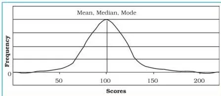
Fig. 2.2 — Positive Skew
In a positive skew the distribution is distorted: the body of the data piles up toward the lower values and a longer tail stretches toward the higher values. The three averages no longer coincide (NCERT, p. 21).
In the standard reading of the figure, the mode lies at the peak of the curve, the median sits a little further along, and the mean is pulled furthest toward the tail by the few very high values — so the order is \( \text{mode} \lt \text{median} \lt \text{mean} \).
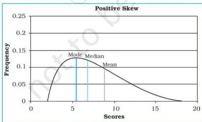
Fig. 2.3 — Negative Skew
The negative skew is the mirror case: the tail stretches toward the lower values while the mass of the data piles up toward the higher values. The three averages separate again (NCERT, p. 21), and the order reverses: \( \text{mean} \lt \text{median} \lt \text{mode} \). The mean is now the value dragged toward the low end of the tail.
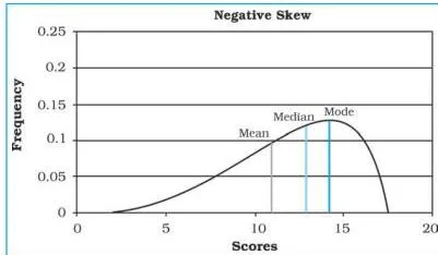
Together, the three figures form the complete pattern: in a normal distribution all three averages are one score at the centre of the bell; in a positive skew they separate with the mode lowest and the mean highest; in a negative skew the order flips.
If you can sketch the bell, the right-hand tail and the left-hand tail, and attach the three averages in the correct order, you have the whole diagram-based answer ready.
Common Mistakes in Mean, Median and Mode (and the Corrections)
The errors below are the ones that actually appear in computation answers for this chapter. Each row gives the mistake, the correct rule, and a way to check yourself.
| Mistake | Correct rule | How to check your answer |
|---|---|---|
| Using \(N/2\) instead of \((N+1)/2\) for the ungrouped median | The median is the \((N+1)/2\)th arranged item | For 7 values the median is the 4th item, not the 3rd |
| Skipping the ascending or descending arrangement before finding the median or mode | Both are defined on an arranged series; arrange first | The list should read from smallest to largest before you locate anything |
| Using class limits such as 20 and 40 instead of the midpoint | Represent each class by its midpoint, (upper + lower)/2 | For class 20–40 the midpoint is 30 — using 20 or 40 shifts the mean |
| Treating \(N\) as the number of classes | \(N\) is the total frequency, \(N = \sum f\) | Add the frequency column; \(N\) is the count of observations, not of rows |
| Dropping the sign when summing \(fd\) in the grouped indirect mean | Add positive and negative \(fd\) values separately, take the absolute difference, and keep the sign of the larger side | If the negative deviations are larger, \(\sum fd\) must come out negative |
| Choosing the wrong median class | The median class is the one whose cumulative frequency is first greater than \(N/2\) | Run down the \(F\) column: your class must be the first \(F\) value above \(N/2\) |
| Swapping \(f\) and \(c\) in the grouped median formula | \(f\) is the frequency of the median class; \(c\) is the cumulative frequency of the pre-median class | \(c\) comes from the row just above the median class, \(f\) from the median class row itself |
| Leaving the unit out of the final answer | Carry the data’s unit: mm, Rs per day, q/ha, m, degrees Celsius | Re-read the question — every value carried a unit, so the answer keeps that unit |
| Declaring a data set without mode too quickly | Check for tied counts before concluding | Two or three ties mean bimodal or trimodal, not without mode |
Answering the Data Processing Exercises with Complete Answers
The chapter closes with six questions and one activity on page 22. Everything needed is inside the chapter itself; below is the ingredient list each complete answer requires. Respect the word lengths the exercise states — about 30 words and about 125 words.
The two multiple-choice questions
Question 1(i): asks which measure of central tendency is not affected by extreme values. A complete answer chooses (d) Median, and the reasoning to carry is: the median is a positional average located by rank in the arranged series, so extreme values cannot move it (NCERT, p. 14).
Question 1(ii): asks for the measure that always coincides with the hump of any distribution. A complete answer chooses (d) Mode, and the reasoning is: the mode is the value of maximum frequency, and the highest-frequency score sits at the hump of a distribution (NCERT, pp. 20-21).
The about-30-words questions
Question 2(i) — define the mean.: A complete answer needs the definition (the value derived by summing all the values and dividing by the number of observations, NCERT p. 13), the formula stated in words (\(\bar{X}\) = sum of observations divided by the number of observations), and one short clause noting that it is the value about which the observations cluster (p. 13).
Question 2(ii) — advantages of using the mode.: A complete answer needs: the mode is identified by inspection after arranging the data (NCERT, p. 20); it gives the most typical, most repeated value; it involves no computation; and it should be balanced by the chapter’s own note that the mode is less widely used than the mean and the median (p. 20).
The about-125-words questions
Question 3(i) — relative positions in normal and skewed distributions, with diagrams.: A complete answer needs the three diagrams (the normal curve, a positive skew, a negative skew); the claim that in a normal distribution the mean, median and mode are the same score because the distribution is symmetrical — highest frequency at the centre, exactly half the scores on each side (NCERT, p. 21); and, for skewed distributions, their separation with the ordering fixed by the tail direction — mode below median below mean for a positive skew, the reverse for a negative skew. The figure walkthrough above rehearses this exact answer.
Question 3(ii) — applicability of the three measures from their merits and demerits.: A complete answer needs one paragraph per average: what each is based on (all values for the mean, rank for the median, frequency for the mode); the kind of geographic data each suits (district rainfall and factory wage groups for the mean, mountain peak heights for the median, student scores for the mode); and each measure’s limitation (the mean is dragged by extreme values, the median ignores the actual size of the values, the mode is less widely used and may be absent or multiple). Keep the three paragraphs tight enough for the 125-word cap.
The closing activity
The activity asks you to take an imaginary example applicable to geographical analysis and explain both the direct and indirect methods of calculating the mean from ungrouped data (NCERT, p. 22).
The complete response needs: a small imaginary geographic data set (six district rainfall values work well), a direct-method computation with \(\bar{X} = \sum x / N\), an indirect-method computation with \(\bar{X} = A + \sum d / N\), and a closing line noting that both give the same mean. Worked Examples 1 and 2 are this activity solved end to end.
Revision Summary — Mean, Median and Mode in One Glance
The whole chapter in one table.
| Measure | Definition | Formula | Key property | Best suited to |
|---|---|---|---|---|
| Mean | Sum of all values divided by the number of observations | \( \bar{X} = \frac{\sum x}{N} \); grouped: \( \bar{X} = \frac{\sum fx}{N} \) | Uses every value; extremes pull it | Fairly balanced data — district rainfall |
| Median | Rank value dividing the arranged series into two equal halves | \( (N+1)/2\)th item; grouped: \( M = l + \frac{i}{f}( \frac{N}{2} – c ) \) | Positional; extremes cannot move it | Skewed data — wages |
| Mode | The most frequently occurring value | None — count frequencies | Found by arrangement and counting; can be more than one | Most common values — repeated peaks or scores |
Two-line recap: in a normal distribution all three averages coincide at the centre of the bell; in a skewed distribution they separate, and the ordering is fixed by the tail direction — \( \text{mode} \lt \text{median} \lt \text{mean} \) for a positive skew, the reverse for a negative skew.
If any method still feels shaky, the worked examples above model each route: Examples 1 and 2 the ungrouped mean, Example 3 the grouped mean, Example 4 the ungrouped median (both odd and even counts), Example 5 the grouped median, and Example 6 the mode.
Before closing, here is where these notes sit. The previous chapter’s Data – Its Source and Compilation notes cover how the raw data were organised for analysis, and the Graphical Representation of Data notes come right after this chapter in the same book.
Both chapters, along with this page, belong to the Class 12 Geography notes hub — and if you need notes for other subjects on the same level, browse the CBSE Class 12 notes section or the main CBSE notes library.
Frequently Asked Questions about Data Processing
Why is the median not affected by extreme values while the mean is?
Because the median is a positional average. It is located by rank in the arranged series, so it is independent of the actual values of the series (NCERT, p. 14). The mean, in contrast, adds every value into its sum, so a single extreme observation changes the total and drags the mean toward it.
The middle rank of the arranged series stays where it was, no matter how large the largest value becomes.
What is the difference between the direct and indirect method of calculating the mean?
The direct method adds the raw values and divides by the number of observations. The indirect method first codes the data — it subtracts an assumed constant \(A\) from every value to create small deviations \(d\) — and then adds the average deviation back: \( \bar{X} = A + \frac{\sum d}{N} \) (NCERT, p. 15).
Coding changes only the size of the numbers, not the average, so both methods give the identical mean; the indirect route is the convenient one when the values are large.
How do I identify the median class when computing a grouped median?
Compute \(N/2\), then move down the cumulative frequency column until you reach the first value greater than \(N/2\). The class that owns this cumulative frequency is the median class (NCERT, p. 19). Its lower limit gives \(l\), its frequency gives \(f\), and the cumulative frequency of the class just above it gives \(c\) for the formula.
Can a data set have more than one mode or no mode at all?
Yes, both are possible. Two values tying for the highest frequency make the set bimodal; three ties make it trimodal; many recurring values make it multimodal; and if no value repeats at all, it is without mode (NCERT, p. 20). A single mode exists only in a unimodal set.
When should I use the mean, median and mode in geography?
Use the mean when the data are fairly balanced and you want one overall representative value, such as the mean rainfall of a group of districts. Prefer the median when extreme values would distort the average — wage data with a few very high figures are the classic case.
Use the mode when you need the most common or typical value, such as the most frequently occurring peak height or temperature. These three uses echo the chapter’s contexts: rainfall and wages for the mean, mountain heights for the median, and test scores for the mode (NCERT, pp. 13-20).
Reference: NCERT Class 12 Practical Work in Geography Part-II textbook, chapter 2 Data Processing.
Explore Class 12 Geography Notes
- Class 12 Geography Notes
- Class 12 CBSE Notes
- CBSE Notes for Classes 1 to 12
- Previous: Data — Its Source and Compilation
- Next: Graphical Representation of Data
Class 12 Geography on LearnCBSE:
Related chapters:
- Spatial Information Technology notes