
These notes cover graphical representation of data, Chapter 3 of the Class 12 Geography textbook Practical Work in Geography, Part-II (NCERT, pp. 23-45).
They follow the 2026-27 session (Rationalised NCERT edition) and compress the chapter into one revision read, ordered the way a teacher would build the skill: why we draw data, which method fits which data, and then how to construct each graph, diagram and map.
The page covers all five diagram forms the chapter constructs — line graphs (including the polygraph), bar diagrams (simple, multiple, compound and combined), pie diagrams, flow maps and the three quantitative thematic maps (dot, choropleth and isopleth) — plus the three formulas, three fully worked examples, a common-mistakes table and answer structure for the chapter’s own exercises.
One clarification up front: this is a revision page. It explains the chapter; it does not carry full solutions to the textbook’s questions or a question bank. You can verify any table, figure or formula against the official NCERT textbook page for Chapter 3.
For the rest of the course, start at the Class 12 Geography notes hub or the wider Class 12 notes collection on the main CBSE notes home.
Why Draw Data? Purpose, Method, Scale and Design
Representation of data is the transformation of data into visual forms such as graphs, diagrams, maps and charts (NCERT, p. 23). Converting a table into a graphic makes patterns visible — population growth, distribution, density, sex ratio, age-sex composition, occupational structure — within a geographical territory. The chapter quotes a Chinese proverb: ‘a picture is equivalent to thousands of words.’
Visuals beat tables for three reasons:
- they make meaningful comparisons between represented phenomena easy;
- they save time — inferences from a table or descriptive text take far longer;
- they leave a longer-lasting impression on the reader’s mind.
Before any diagram is drawn, three planning decisions fix the result (NCERT, p. 24):
| Decision | What it means | Chapter example |
|---|---|---|
| Suitable method | Match the data’s character to an appropriate graphical method. | Temperature or population growth over time — line graph; rainfall or commodity production — bar diagram; population or livestock distribution — dot map; population density — choropleth map. |
| Suitable scale | The scale is the measure of data on the diagram or map; it must fit the entire data set. | ‘The scale should neither be too large nor too small’ (NCERT, p. 24). |
| Design | Cartographic design components shown on the finished diagram or map. | Title (area + year + caption) top centre; legend or index lower left or right; North direction symbol on maps. |
Cartographic design links this chapter to ‘Essentials of Map Making’, Chapter 1 of the Class XI Practical Work in Geography, Part-I (NCERT, 2006). The data themselves are prepared earlier in this same book — in Chapter 1, covered in the Data: Its Source and Compilation notes.
Matching Data to the Right Method and Map
Choosing the right visual for a given data set is the most reusable skill in this chapter. NCERT fixes these data-to-method pairings on p. 24:
| Kind of data | Recommended method |
|---|---|
| Temperature or population growth over time | Line graph |
| Rainfall or production of commodities | Bar diagram |
| Distribution of population (human or livestock), or crop-producing areas | Dot map |
| Population density | Choropleth map |
Diagrams are also classified by dimension (NCERT, pp. 24-25):
| Class | Members |
|---|---|
| One-dimensional | Line graph, polygraph, bar diagram, histogram, age-sex pyramid |
| Two-dimensional | Pie diagram, rectangular diagram |
| Three-dimensional | Cube and spherical diagrams |
The chapter then names the five forms it calls ‘most commonly drawn’: line graphs, bar diagrams, pie diagram, wind rose and star diagram, and flow charts. Wind rose and star diagrams are only named, never constructed, so you need their names and their family — not a construction procedure.
Diagrams have a built-in limit: they compare internal variations within data but fail to give a regional perspective (NCERT, pp. 35-36). That gap is filled by distribution maps — dot, choropleth and isopleth — which show how a phenomenon varies across space. This is why the chapter has two halves: diagrams for internal comparison, maps for spatial pattern.
Line Graphs and Polygraphs: Change Over Time
A line graph represents time-series data — temperature, rainfall, population growth, birth rates and death rates (NCERT, p. 25). Construction takes four steps:
- Simplify the data into round numbers before plotting.
- Draw the axes: time goes on the X-axis, the plotted value on the Y-axis.
- Choose and label the Y-scale; when the data contain a negative figure, the scale must show it — exactly what Fig. 3.1 demonstrates.
- Plot, mark and join: place each year’s value as a dot and join the dots with a freehand line.
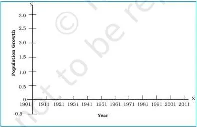
In Fig. 3.1 the Y-axis scale is extended below zero so that a negative growth value can be plotted without distortion — the detail that makes the 1921 dip in population growth visible when Example 3.1 is drawn.
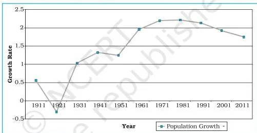
Example 3.1 produces Fig. 3.2, the annual growth of population in India from 1901 to 2011. Reading the line: growth dips below zero in 1921 and peaks in the early 1980s — both facts sit directly in Table 3.1 (1921: -0.30; 1981: 2.22).
The textbook’s Activity on p. 26 asks you to find the reason for the sudden change between 1911 and 1921 shown in Fig. 3.2. The chapter leaves it open.
The historically accepted cause is the influenza pandemic of 1918-19; that explanation is outside the NCERT text itself, so treat it as a research hint and confirm it from a reliable history source before using it in an answer.
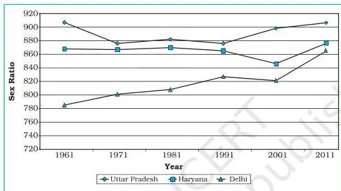
A polygraph is a line graph in which two or more variables are shown by an equal number of lines for immediate comparison (NCERT, p. 26). Example 3.2 compares the sex ratio of Delhi, Haryana and Uttar Pradesh from 1961 to 2011; in Fig. 3.3 each state’s line uses a different pattern — straight, broken, dotted, or dot-and-dash — or a different colour.
Bar Diagrams: Simple, Multiple, Compound and Combined
A bar diagram, also called a columnar diagram, is drawn with columns of equal width. Three rules govern the whole family (NCERT, p. 27):
- all bars have the same width;
- all bars sit at equal intervals;
- bars may be shaded or patterned to keep them distinct.
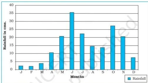
Simple bar diagram (Example 3.3). Built for an immediate comparison of one variable. Non-time data are arranged in ascending or descending order before plotting; time-series data keep their chronological sequence. In Fig. 3.4, Thiruvananthapuram’s average monthly rainfall is drawn by dividing the X-axis into 12 equal month parts and scaling rainfall in cm on the Y-axis.
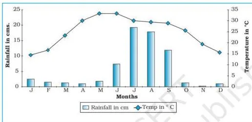
Combined line-and-bar graph (Example 3.4). Two closely connected measures — mean monthly temperature and rainfall — are drawn as one diagram: months on the X-axis, temperature scaled on the right of the Y-axis and drawn as a line, rainfall scaled on the left and drawn as bars. Fig. 3.5, the Delhi climate graph, is the standard climate-diagram style.
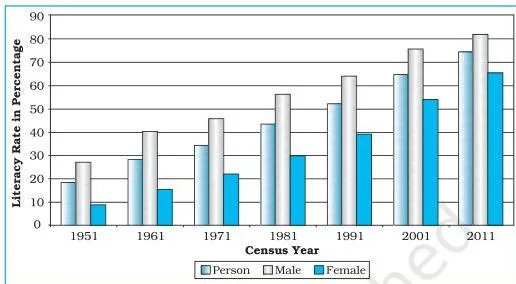
Multiple bar diagram (Example 3.5). Represents two or more variables for comparison — for instance the literacy of the total, male and female population. Each year’s values are drawn as closed columns next to one another (Fig. 3.6).
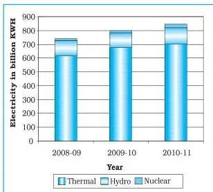
Compound bar diagram (Example 3.6). Represents the components of one total: different components are grouped into a single bar as separate rectangles. In Fig. 3.7, one bar per year shows gross electricity generation, divided into its thermal, hydro and nuclear segments.
The four forms students most often mix up are compared below — the chapter’s own exercise asks for exactly this distinction:
| Method | What it represents | Construction signature | Chapter example |
|---|---|---|---|
| Polygraph | Two or more time-series variables | Separate line patterns in one graph | Sex ratio of Delhi, Haryana, UP (Fig. 3.3) |
| Multiple bar | Two or more variables compared | Bars placed side by side | Literacy by total, male, female (Fig. 3.6) |
| Compound bar | Components of one total | Single bar split into segments | Electricity by thermal, hydro, nuclear (Fig. 3.7) |
| Combined line-and-bar | Two related measures together | Temperature line plus rainfall bars, two Y-scales | Delhi climate (Fig. 3.5) |
Pie Diagram: Dividing the Circle Into Degrees
A pie diagram — NCERT’s alternative name is divided circle diagram — draws the total value of an attribute as a circle, then divides the circle into angles that represent the sub-sets of the data (NCERT, p. 31). Think of a pizza or a cake: the whole circle is the total, and each slice’s angle is proportional to its share.
The angle for each component is:
\[ \text{Angle of a component} = \frac{\text{Component value}}{\text{Total value}} \times 360^\circ \]
When the data are already percentages, the chapter uses:
\[ \text{Angle} = \frac{\text{Percentage} \times 360}{100} = \text{Percentage} \times 3.6 \]
The constant 3.6 exists because a circle has 360° and the percentages total 100: \(360 \div 100 = 3.6\) (NCERT, p. 31).
Construction follows four steps (NCERT, p. 32):
- Choose a radius of 3, 4 or 5 cm.
- Draw a line from the centre of the circle to the arc as a radius.
- Measure the angles from the arc, clockwise, in ascending order — starting from the smaller angle.
- Complete the diagram with a title, sub-title and legend, using distinct shades or colours for each category.
Two precautions apply (NCERT, p. 32):
- The circle must be neither too big to fit the space nor too small to be legible.
- Starting with the biggest angle accumulates error and makes the smallest angle hard to plot — always start small.
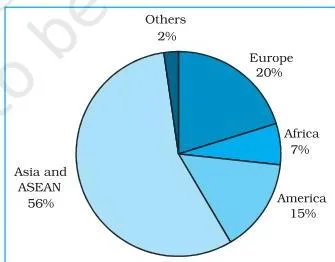
Example 3.7 draws the direction of Indian exports in 2010-11 as Fig. 3.8. The largest slice — Asia and ASEAN, at 56.2% of exports — is visible immediately, which is exactly the ‘lasting impression’ a well-made pie leaves.
Flow Maps: Movement Drawn With Proportional Lines
A flow map (or flow chart) is a combination of graph and map. It shows the movement of commodities or people between places of origin and destination, and the chapter calls it a dynamic map (NCERT, p. 33). Flow maps are drawn with lines of proportional width — the thicker the strip, the larger the flow.
They handle two kinds of data (NCERT, p. 33):
- the number and frequency of vehicles by direction of movement;
- the number of passengers or the quantity of goods transported.
Three things are required:
- a route map showing the transport routes with connecting stations;
- flow data (goods, services, vehicles) with the origin and destination of each movement;
- a scale through which the quantity or number is represented.
Example 3.8 applies this to train traffic around Delhi. In the data set the maximum is 50 trains (Old Delhi-New Delhi) and the minimum is 6 (Udyog Nagar-Tikri Kalan). With a scale of 1 cm = 50 trains, the busiest route becomes a strip \(\frac{50}{50} \times 10\ \text{mm} = 10\ \text{mm}\) thick and the quietest just \(\frac{6}{50} \times 10\ \text{mm} = 1.2\ \text{mm}\).
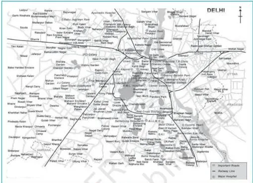
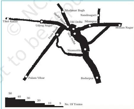
The pair of figures shows the process: Fig. 3.9 is the plain outline map of Delhi with its railway lines and nodal stations — the input — and Fig. 3.10 is the finished traffic flow map, where each route carries a strip whose thickness follows the scale.
A terraced scale is added as the legend, and nodal stations are marked with a distinct symbol (NCERT, p. 34).
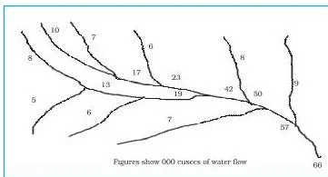
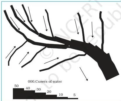
Example 3.9 repeats the idea for water: the base Ganga Basin map (Fig. 3.11) is converted into a flow map by drawing strips whose width represents discharge, and the chapter fixes 1 cm width = 50,000 cusecs of water for the construction (Fig. 3.12).
You have seen this tool outside the classroom: metro route maps and railway traffic-density maps published by transport authorities use exactly the same proportional-line logic.
Thematic Maps: Dot, Choropleth and Isopleth
Graphs and diagrams compare internal variations within data, but they fail to produce a regional perspective — the view of how a characteristic spreads across space (NCERT, pp. 35-36). Maps that show this are called thematic maps or distribution maps.
Making one requires three things (NCERT, p. 36):
- state- or district-level data on the chosen theme;
- an outline map of the study area with administrative boundaries;
- a physical map of the region — a physiographic map for population distribution, a relief and drainage map for transport.
The final map must also carry five design components: name of the area; title of the subject matter; source of the data and year; indication of symbols, signs, colours and shades; and the scale (NCERT, p. 36).
Thematic maps split into two classes. Quantitative (statistical) maps show measurable variation — say, areas receiving more than 200 cm, 100 to 200 cm, 50 to 100 cm and less than 50 cm of rainfall. Non-quantitative (qualitative) maps show non-measurable characteristics, such as a map of ‘high rainfall’ versus ‘low rainfall’ areas (NCERT, p. 36). This chapter constructs only the quantitative trio: dot, choropleth and isopleth maps.
These are the maps you already see daily: the temperature bands and pressure lines on newspaper and TV weather maps belong to this family. The rest of the practical course extends these map skills further; the Class 12 Geography hub indexes the related chapter notes, including spatial information technology.
Dot Maps: Distribution Through Dots of Equal Size
A dot map shows the distribution of phenomena such as population, cattle and crops. Dots of the same size, each worth a fixed value fixed by a scale, are marked over administrative units to reveal distribution patterns (NCERT, p. 36).
The four requirements (NCERT, p. 36):
- an administrative map showing state, district or block boundaries;
- statistical data on the theme for each administrative unit;
- a scale that determines the value of one dot;
- a physiographic map of the region, especially relief and drainage maps.
Two precautions (NCERT, p. 37):
- boundary lines must not be very thick or bold;
- all dots must be the same size.
The dot count for a unit is the total population divided by the value of one dot. For Maharashtra, with the scale fixed at 100,000 people per dot (NCERT, p. 39):
\[ \frac{96,752,247}{100,000} = 967.52 \approx 968\ \text{dots} \]
— rounded up to 968 because the fraction exceeds 0.5. Take an original mini-example: a district with a population of 12,50,000 and a dot value of 50,000 takes \(\frac{12,50,000}{50,000} = 25\) dots.
Finally, the physiographic map guides placement: fewer dots are marked over mountainous, desert and snow-covered areas (NCERT, p. 39).
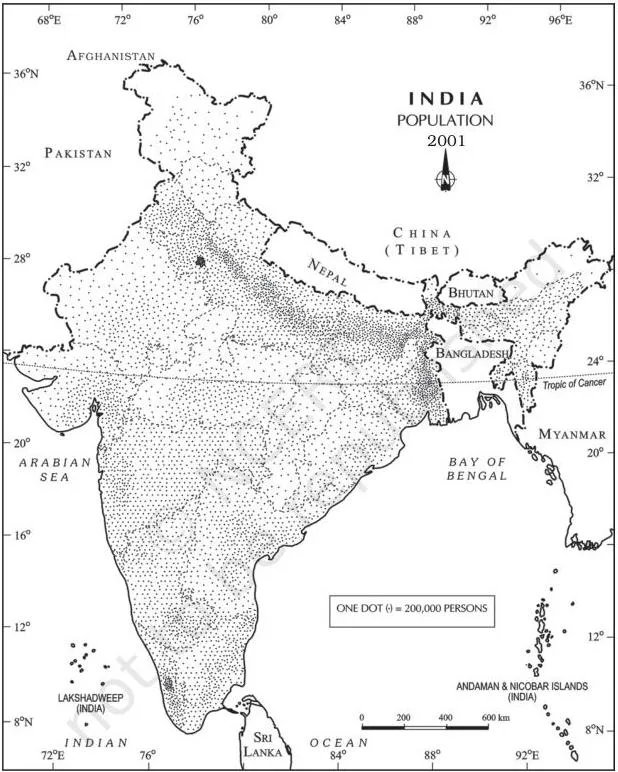
Fig. 3.13 (Population of India, 2001) shows this logic at national scale: compare Uttar Pradesh’s dense dot field with the near-empty mountain states — that contrast is the map’s whole message.
Choropleth Maps: Shading Administrative Units
A choropleth map represents data that belong to administrative units — states or districts — using shades or patterns. It is the standard tool for population density, literacy or growth rates, and sex ratio (NCERT, p. 39).
The steps run in teaching order (NCERT, pp. 39-41):
- Arrange the data in ascending (or descending) order.
- Group the data into five categories: very high, high, medium, low and very low.
- Fix the interval with \(\text{Interval} = \frac{\text{Range}}{5}\), where \(\text{Range} = \text{maximum value} – \text{minimum value}\).
- Assign shades or patterns in increasing or decreasing order of intensity.
- Complete the map with the design attributes — title, legend, scale, source and year.
Example 3.11 works through the numbers. The lowest literacy rate is Bihar’s 47% and the highest is Kerala’s 90.9%; the chapter rounds 90.9 to 91.0 for the range, giving (NCERT, p. 39):
\[ \text{Range} = 91.0 – 47.0 = 44.0; \qquad \text{Interval} = \frac{44.0}{5} = 8.8 \approx 9.0 \]
Adding 9.0 successively to 47.0 builds five bands: 47-56, 56-65, 65-74, 74-83 and 83-92, labelled very low through very high.
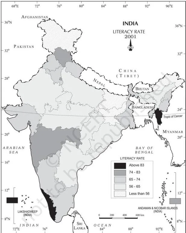
Fig. 3.14 shades each category from light to dark, and the south-versus-north literacy contrast is readable at a glance — the spatial reading a choropleth exists to give.
Isopleths and Interpolation: Lines of Equal Value
Some data are continuous — temperature, rainfall, slope — and vary across natural boundaries rather than administrative ones. These are drawn with isopleths: the word comes from ‘iso’ (equal) and ‘pleth’ (line), so an isopleth is an imaginary line joining places of equal value (NCERT, p. 42).
| Isopleth | Shows |
|---|---|
| Isotherm | Equal temperature |
| Isobar | Equal pressure |
| Isohyet | Equal rainfall |
| Isoneph | Equal cloudiness |
| Isohel | Equal sunshine |
| Contour | Equal height |
| Isobath | Equal depth |
| Isohaline | Equal salinity |
Memory device: therm = heat, bar = pressure, hyet = wet (rhymes with wet), neph = clouds, hel = sun (helios), bath = deep (bathys), haline = salt.
Drawing rules (NCERT, p. 42):
- choose an equal interval between lines;
- intervals of 5, 10 or 20 are ideal;
- write the value along the line, in the middle, breaking the line to do so.
The requirements are a base map showing point locations, data of temperature, pressure or rainfall over a definite period, and drawing instruments — especially a French curve (NCERT, p. 42).
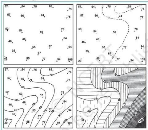
Interpolation inserts intermediate values between the observed values at two stations — for example between the temperatures at Chennai and Hyderabad or between two spot heights. Generally, drawing isopleths that join places of the same value is itself called interpolation. The exact point of an isopleth is found by (NCERT, p. 42):
\[ \text{Point of isopleth} = \frac{\text{Distance between two points (cm)}}{\text{Difference between their values}} \times \text{Interval} \]
The chapter’s own worked case: two places record \(28^\circ\text{C}\) and \(33^\circ\text{C}\), and the \(30^\circ\text{C}\) isotherm is to be drawn. The distance between the two points is 10 mm and the value difference is \(33 – 28 = 5\). The target value 30 is 2 units away from 28, so (NCERT, p. 43):
\[ \frac{10\ \text{mm}}{5} \times 2 = 4\ \text{mm} \]
The \(30^\circ\text{C}\) isotherm is plotted 4 mm from the \(28^\circ\text{C}\) point — or, equivalently, 6 mm from the \(33^\circ\text{C}\) point, because \(10 – 4 = 6\). Draw the minimum-value isopleth first, then the rest (NCERT, p. 43).
Every weather forecast you watch uses this family: the isobars on the pressure chart are isopleths of pressure. Once you recognise the names, the chapter’s terms become the familiar symbols of the forecast map.
Definitions You Must Know: From ‘Representation’ to ‘Isopleth’
| Term | Meaning | Example in this chapter |
|---|---|---|
| Representation of data | Converting data into visual forms such as graphs, diagrams, maps and charts. | Population growth or sex-ratio patterns become visible (p. 23). |
| Line graph | A graph for time-series data, with time on the X-axis and the value on the Y-axis. | Annual growth of population, 1901-2011 (p. 25). |
| Polygraph | A line graph with two or more variables drawn with an equal number of lines. | Sex ratio of Delhi, Haryana and UP (p. 26). |
| Bar diagram / columnar diagram | Columns of equal width placed at equal intervals. | Average monthly rainfall of Thiruvananthapuram (p. 27). |
| Simple bar diagram | A single variable plotted for immediate comparison. | Monthly rainfall, Example 3.3 (p. 27). |
| Multiple bar diagram | Two or more variables compared by bars placed side by side. | Total, male and female literacy (p. 29). |
| Compound bar diagram | Components of one total shown as segments of a single bar. | Electricity as thermal, hydro and nuclear (p. 30). |
| Pie diagram / divided circle diagram | A circle divided into angles proportional to each component’s share. | Direction of Indian exports, 2010-11 (p. 31). |
| Flow map / chart / dynamic map | A graph-map combination showing movement between origin and destination by proportional line width. | Railway traffic flow map of Delhi (p. 33). |
| Thematic map / distribution map | A map showing the regional distribution of a phenomenon over space. | Literacy rate across states (pp. 35-36). |
| Quantitative (statistical) map | Shows measurable variation, such as rainfall classed into totals. | The dot-choropleth-isopleth trio (p. 36). |
| Non-quantitative (qualitative) map | Shows non-measurable characteristics, such as high- versus low-rainfall areas. | ‘High rainfall’ vs ‘low rainfall’ map (p. 36). |
| Dot map | Equal-size dots, each worth a fixed value, marked over administrative units. | Population of India, 2001 (p. 36). |
| Choropleth map | Administrative units shaded by data classes. | Literacy rate of India, 2001 (p. 39). |
| Isopleth | An imaginary line joining places of equal value. | Isotherms, isobars, isohyets (p. 42). |
| Interpolation | Inserting intermediate values between observed values at two stations. | Fixing the \(30^\circ\text{C}\) isotherm between \(28^\circ\text{C}\) and \(33^\circ\text{C}\) (p. 42). |
| Legend or index | Explains the colours, shades, symbols and signs used in a map or diagram. | Positioned lower left or right of the map (p. 24). |
| Scale | The measure by which data values are converted to diagram or map distances. | 1 cm = 50 trains in the Delhi flow map (p. 24). |
| Title and direction | Design components: a title naming the area, year and caption; a North symbol on maps. | Both placed on the final diagram or map (p. 24). |
The Chapter’s Three Formulas: Angles, Intervals, Interpolation
Only three formulas appear in this chapter, and all three are used again in the worked examples below.
| Formula | Written form | What it gives |
|---|---|---|
| Pie angle (values) | \( \frac{\text{Component value}}{\text{Total value}} \times 360^\circ \) | Angle of one component, in degrees |
| Pie angle (percentages) | \( \frac{\text{Percentage} \times 360}{100} = \text{Percentage} \times 3.6 \) | Angle directly from a percentage |
| Choropleth interval | \( \frac{\text{Maximum value} – \text{Minimum value}}{5} \) | Width of one of the five categories |
| Point of isopleth | \( \frac{\text{Distance between two points (cm)}}{\text{Difference between their values}} \times \text{Interval} \) | Distance in cm or mm from one station toward the other |
The constant 3.6 is the full angle of a circle divided by 100 percentage points: \(360 \div 100 = 3.6\) (NCERT, p. 31). Units: pie angles come out in degrees; choropleth intervals carry the unit of the original data (percent, persons per square km, and so on); the isopleth point is a distance measured on the map.
For interpolation, the chapter’s method first finds the minimum and maximum values, calculates the range, then chooses a whole-number interval such as 5, 10 or 15 before applying the formula (NCERT, p. 42).
Worked Examples: From Data to Finished Diagram
Each example below uses fresh numbers, not the textbook’s values, so you can follow the calculation itself. The method and rule are named first, then every step is shown with its units.
Example 1: Pie Diagram Angles From Percentages
Method: pie diagram using the constant 3.6. Rule: each percentage times 3.6 gives the angle, and the rounded angles must sum to 360° (NCERT, p. 31).
Illustrative data — share of India’s iron-ore production by state: Odisha 52%, Chhattisgarh 21%, Karnataka 20%, Others 7%.
Step 1: Verify the percentages total 100: \(52 + 21 + 20 + 7 = 100\).
Step 2: Multiply each percentage by 3.6.
\[ \text{Odisha: } 52 \times 3.6 = 187.2 \approx 187^\circ \]
\[ \text{Chhattisgarh: } 21 \times 3.6 = 75.6 \approx 76^\circ \]
\[ \text{Karnataka: } 20 \times 3.6 = 72^\circ \]
\[ \text{Others: } 7 \times 3.6 = 25.2 \approx 25^\circ \]
Step 3: Check that the rounded angles sum to 360°: \(187 + 76 + 72 + 25 = 360^\circ\).
Step 4: Arrange the slices in ascending order — 25°, 72°, 76°, 187° — and plot clockwise from the smallest angle, exactly as the chapter’s construction demands.
Step 5: Finish with a title, sub-title and legend using distinct shades for each state.
Final answer: Odisha 187°, Chhattisgarh 76°, Karnataka 72°, Others 25° — summing to 360°. This is exactly the structure NCERT uses in Table 3.7(b) on pp. 31-32.
Example 2: Locating an Isopleth by Interpolation
Method: interpolation formula. Rule: point of isopleth = (distance between two points ÷ difference of their values) × interval (NCERT, p. 42).
Original values: station A records \(16^\circ\text{C}\), station B records \(22^\circ\text{C}\); the isotherm to draw is \(18^\circ\text{C}\); the distance between the stations on the map is 15 mm.
Step 1: Find the interval — the gap between the target value and the lower station value: \(18 – 16 = 2\).
Step 2: Find the difference between the two station values: \(22 – 16 = 6\).
Step 3: Apply the formula:
\[ \frac{15\ \text{mm}}{6} \times 2 = 5\ \text{mm} \]
Step 4: So the \(18^\circ\text{C}\) isotherm passes 5 mm from station A toward B.
The remaining distance from station B is \(15 – 5 = 10\ \text{mm}\), so the placement checks on both sides.
Step 5: Draw the minimum-value isopleth first, then add this one (NCERT, p. 43).
Final answer: The \(18^\circ\text{C}\) isotherm lies 5 mm from station A (and 10 mm from station B).
Example 3: Building Choropleth Categories From the Range
Method: choropleth class interval. Rule: interval = range ÷ 5, where range = maximum − minimum (NCERT, p. 39).
Original values: literacy rates across 20 districts of a state range from a minimum of 52% to a maximum of 92%.
Step 1: Find the range: \(92 – 52 = 40\).
Step 2: Divide by 5: \(40 \div 5 = 8\).
Step 3: Add 8 successively to the minimum to build five bands: 52-60, 60-68, 68-76, 76-84, 84-92.
Step 4: Label the bands very low, low, medium, high and very high.
Step 5: Shade from the lightest tone (very low) to the darkest (very high), then add the map-design attributes.
Contrast: NCERT’s Example 3.11 rounded 8.8 up to 9.0 because 44.0 ÷ 5 does not divide cleanly; this example used 40 ÷ 5 = 8 so the mechanism is easier to see.
Both follow the same rule.
Final answer: Five classes of width 8 — 52-60, 60-68, 68-76, 76-84, 84-92 — shaded from light to dark.
Common Mistakes in Diagram Construction
| Students write or do | Correct is | How to check your answer |
|---|---|---|
| Time on the Y-axis and values on the X-axis. | In time-series graphs, time always goes on the X-axis and the value on the Y-axis (p. 25). | Check the two axes against the rule before plotting. |
| Bars of unequal width or uneven gaps. | All bars have equal width and sit at equal intervals (p. 27). | Measure a few bar widths and gaps. |
| Pie sectors measured starting from the largest angle. | Start from the smaller angle; a big starting angle accumulates error and leaves the smallest angle hard to plot (p. 32). | Check that the smallest angle plots cleanly. |
| Rounded pie degrees that do not sum to 360°. | After rounding, adjust so the angles total 360° — the chapter’s Table 3.7(b) ends at exactly 360°. | Add the rounded angles; if the sum is off, fix the largest angle. |
| A choropleth drawn with only four classes, or without dividing the range by 5. | Always form five categories (very high to very low) using Range ÷ 5 (p. 39). | Count the bands; there should be five. |
| Dot maps with different dot sizes, or dots spaced uniformly. | All dots are the same size, and fewer dots are placed over mountains, deserts and snow as the physiographic map advises (pp. 37, 39). | Compare dot sizes; check relief areas have fewer dots. |
| Interpolation done as distance ÷ difference without multiplying by the interval. | The formula is (distance ÷ difference) × interval — the multiplier is essential, e.g. \(\frac{10}{5} \times 2 = 4\ \text{mm}\) (p. 43). | Substitute the numbers back into the full formula. |
| Isopleth lines drawn crossing one another. | Lines of equal value can never cross; each isopleth traces a single value. | Check that no two lines intersect. |
| Confusing multiple and compound bar diagrams. | Multiple bars sit side by side to compare variables; a compound bar is one bar segmented into components of a total (pp. 29-30). | Ask: am I comparing variables or dissecting one total? |
| A scale too large or too small for the data. | The scale must fit the entire data set — neither too large nor too small (p. 24). | Plot the maximum value; it must fit on the page. |
Exam Notes: Writing Complete Answers to the Chapter Exercises
Choose-the-right-answer items (p. 43). Four one-line reasoning points:
- Population distribution — dot maps, because the chapter pairs the distribution of population (and livestock) with dot maps (p. 24).
- Decadal growth of population — line graph, because growth over successive decades is time-series data (pp. 24-25).
- Polygraph — drawn for more than two variables, by its definition of an equal number of lines for two or more variables (p. 26).
- ‘Dynamic Map’ — flow map, the name NCERT gives the flow map on p. 33.
Short questions (p. 44). A complete answer needs these points:
- Thematic map: definition (a map showing the regional distribution of a phenomenon over space) + why it is drawn (graphs lack a regional perspective) + one example.
- Multiple vs compound bar: two clear differences — multiple bars sit side by side to compare variables; a compound bar is a single bar split into segments that are components of one total (pp. 29-30).
- Dot-map requirements: the four requirements of p. 36 — administrative map with boundaries, statistical data per unit, a scale fixing the value of a dot, and a physiographic map.
- Traffic flow map method: the sequence of Example 3.8 — take the route map with nodal stations, select a scale (1 cm = 50 trains), plot each route’s strip thickness, then add a terraced legend and a nodal symbol (pp. 33-34).
- Isopleth and interpolation: define both, write the interpolation formula, and give the 28 °C to 33 °C case as a one-line example.
- Choropleth steps: the seven-step sequence — arrange data, find the range, divide by 5, form the five bands, assign shades in order, prepare the map, complete the design (pp. 39-41).
- Pie-diagram steps: the four construction steps plus the two precautions on p. 32.
Activity data sets (pp. 44-45). The chapter ends with five practice data sets; each points to a method:
| Data set | Method to choose |
|---|---|
| Urbanisation trends, 1901-2001 (decennial growth %) | Line graph — a time series |
| Literacy and enrolment ratios (person, male, female; boys, girls) | Multiple bar diagram — several variables to compare |
| Land use, 1950-51 vs 1998-2001 (six land-use categories) | Pie diagram — shares of a total |
| Rice area and production by state | Multiple bar for area, pie for the percentage of area, dot map for production, choropleth for the percentage of production |
| Kolkata monthly temperature and rainfall | Combined line-and-bar graph |
Constructing these diagrams assumes the data have already been processed — that is Chapter 2, covered in the data processing notes, the step that precedes representation.
Revision Recap: Diagram by Diagram
Everything above condenses into the decision table below — the one screen to scan the night before your exam.
| Data situation | Method | Key construction rule | Chapter example |
|---|---|---|---|
| Temperature or growth over time | Line graph | Time on X, value on Y, dots joined freehand; Y-scale must show negatives | Example 3.1, Fig. 3.2 |
| Two or more variables over time | Polygraph | One line pattern per variable | Example 3.2, Fig. 3.3 |
| One variable’s values, e.g. monthly rainfall | Simple bar | Equal width, equal intervals; non-time data arranged ascending or descending | Example 3.3, Fig. 3.4 |
| Climate data — temperature plus rainfall | Combined line-and-bar | Temperature line on the right Y-scale, rainfall bars on the left | Example 3.4, Fig. 3.5 |
| Two or more variables compared, e.g. literacy by sex | Multiple bar | Bars side by side | Example 3.5, Fig. 3.6 |
| Components of a total, e.g. electricity by source | Compound bar | One bar, segmented into components | Example 3.6, Fig. 3.7 |
| Share of a total, e.g. export destinations | Pie diagram | Angles via the 3.6 constant; plot from the smaller angle clockwise | Example 3.7, Fig. 3.8 |
| Movement along routes, e.g. trains | Flow map | Strip width proportional to quantity; terraced scale legend | Examples 3.8, 3.9; Figs. 3.9-3.12 |
| Distribution of a phenomenon, e.g. population | Dot map | Dots of equal value; fewer dots over mountains, deserts and snow | Example 3.10, Fig. 3.13 |
| Rate or density per administrative unit | Choropleth | Five classes built from Range ÷ 5 | Example 3.11, Fig. 3.14 |
| Continuous fields — temperature, pressure, rainfall | Isopleth | Lines of equal value; interpolation formula for each line | p. 42, Fig. 3.15 |
- Dimension classification: 1-D (line, polygraph, bar, histogram, age-sex pyramid); 2-D (pie, rectangular); 3-D (cube, sphere).
- Map split: quantitative (statistical) vs non-quantitative (qualitative) thematic maps; this chapter constructs only the quantitative trio.
- Iso-family memory hook: therm = heat, bar = pressure, hyet = wet, neph = clouds, hel = sun, bath = deep, haline = salt.
Frequently Asked Questions
Which diagram is best for temperature data and which for rainfall?
Use a line graph for temperature (a time series) and a bar diagram for rainfall (NCERT, p. 24). When both must appear together — as in a climate graph — combine them into one line-and-bar graph with months on the X-axis, temperature drawn as a line on the right scale and rainfall as bars on the left (p. 28).
What is the difference between a multiple bar diagram and a compound bar diagram?
A multiple bar diagram places two or more variables side by side — separate bars per variable, for comparison. A compound bar diagram draws one bar for the total and divides that single bar into rectangular segments, each a component of the total (NCERT, pp. 29-30). Multiple bars compare separate variables; compound bars dissect one total.
How do I calculate pie diagram angles when the data are in percentages?
Multiply each percentage by 3.6: \(\text{angle} = \text{percentage} \times 3.6\) (NCERT, p. 31). Round each angle to the nearest degree, then check that the rounded angles sum to 360° — if not, adjust the largest angle by the difference.
What is the difference between a dot map and a choropleth map?
A dot map uses equal-size dots, each worth a fixed value, to show the distribution of actual quantities such as population or cattle; the physiographic map decides where dots are thinned out. A choropleth map instead shades whole administrative units by data classes such as density or literacy rate (NCERT, pp. 36, 39).
Dots place quantities; choropleths shade rates or densities per unit of area.
How does the isopleth interpolation formula work?
The formula places a line of equal value between two stations (NCERT, p. 42):
\[ \text{Point of isopleth} = \frac{\text{Distance between two points (cm)}}{\text{Difference between their values}} \times \text{Interval} \]
In the chapter’s own case, a \(30^\circ\text{C}\) isotherm between \(28^\circ\text{C}\) and \(33^\circ\text{C}\), 10 mm apart, sits \(\frac{10}{5} \times 2 = 4\ \text{mm}\) from the \(28^\circ\text{C}\) point (p. 43).
Why is the 1911-1921 population growth negative in Fig. 3.2?
The NCERT text does not answer this — it sets the question as an Activity on p. 26. The historically accepted reason is the influenza pandemic of 1918-19. That explanation is not in the NCERT text, so treat it as a research hint and confirm it from a reliable history source before using it in an answer.
Reference: NCERT Class 12 Geography textbook, chapter Graphical Representation of Data.
Explore Class 12 Geography Notes
- Class 12 Geography Notes
- Class 12 CBSE Notes
- CBSE Notes for Classes 1 to 12
- Previous: Data Processing
- Next: Spatial Information Technology
Class 12 Geography on LearnCBSE:
Related chapters:
- Data — Its Source and Compilation notes
Official source: download the NCERT textbook free from ncert.nic.in.