
Market equilibrium class 12 — this page carries the official NCERT Class 12 Economics Chapter 5 PDF for Introductory Microeconomics, the chapter titled Market Equilibrium. The chapter runs about twenty printed pages and answers one question: how market demand and market supply together settle on the price and quantity that clear a perfectly competitive market.
The official PDF is directly below, and the rest of the page explains, section by section, what the chapter teaches once you open it. This page is maintained for the 2026-27 session.
| What the chapter holds | Count | Where it is used |
|---|---|---|
| Printed pages | 20 | |
| Sections in the chapter | 6 | |
| Figures with NCERT captions | 11 | |
| Tables | 1 | |
| Worked examples | 2 | solved step by step in our NCERT Solutions |
| Exercise questions | 25 | answered in our NCERT Solutions |
| Official NCERT PDF | Download the chapter PDF | the chapter exactly as NCERT publishes it |
Market Equilibrium Class 12 Economics Chapter 5 PDF
The official Market Equilibrium Class 12 Economics Chapter 5 PDF is the fifth chapter of NCERT’s Introductory Microeconomics, published on the NCERT portal where you can verify the edition and download the complete textbook.
The chapter occupies roughly twenty pages of the printed book — from page 71, where equilibrium is defined, to the applications of demand-supply analysis in the price ceiling and price floor sections, and finally the exercises and glossary. Open the PDF to read the chapter in its original layout, with every figure and table placed where the text refers to it.
What Is Inside the Market Equilibrium Chapter
The table below lists what the chapter holds — its sections, diagrams, worked examples and exercise questions — so you can see the scale of the file before opening it. Use it to check whether you have worked through everything the chapter contains.
As for what the chapter teaches: it opens with the meaning of equilibrium and the twin states of excess demand and excess supply, builds two models of a perfectly competitive market — one with a fixed number of firms, one with free entry and exit — then detours through the labour market before applying the framework to price controls.
Two worked examples, 5.1 and 5.2, demonstrate the method on a wheat market, and the chapter closes with exercises and a glossary.
Where the Chapter Goes: From Equilibrium to Price Controls
This roadmap maps each block of the chapter to its page in the printed book, so you can jump straight to the part that is confusing you.
| Block of the chapter | Printed pages | What it does |
|---|---|---|
| Equilibrium, excess demand, excess supply | p. 71 | Defines equilibrium as matching plans that clear the market; introduces \( p^* \), \( q^* \), excess demand and excess supply (NCERT p. 71) |
| Out-of-equilibrium behaviour | p. 72 | Adam Smith’s invisible hand: price rises with excess demand, falls with excess supply (NCERT p. 72) |
| Market equilibrium: fixed number of firms | pp. 72–74 | Equilibrium at the intersection of market demand \( DD \) and market supply \( SS \), with Example 5.1 (NCERT pp. 72–74) |
| Wage determination in the labour market | pp. 74–76 | Firms hire until \( w = MRP_L \); backward-bending individual labour supply (NCERT pp. 74–76) |
| Shifts in demand and supply | pp. 76–80 | Direction rules for demand and supply shifts; Table 5.1 on simultaneous shifts (NCERT pp. 76–80) |
| Market equilibrium: free entry and exit | pp. 80–83 | Price equals minimum average cost; Example 5.2; demand shifts change quantity but not price (NCERT pp. 80–83) |
| Applications: price ceiling and price floor | pp. 84–85 | Government price controls and their consequences (NCERT pp. 84–85) |
| Exercises and glossary | p. 86 onward | Revision questions, numericals and the book’s glossary (NCERT p. 86) |
The order matters: the chapter combines the market demand curve of Chapter 2 with the market supply curve of Chapter 4 and asks where the two plans match. Once you see that intersection, every later section — shifts, entry and exit, price controls — is a variation on it.
Key Concepts in Market Equilibrium
This chapter answers a single question: at what price does the quantity buyers want equal the quantity sellers want to supply, and what pulls the market to that price? Each subsection below is one building block of that answer.
Equilibrium, Excess Demand and Excess Supply
An equilibrium is a situation where the plans of all consumers and firms in the market match and the market clears: the aggregate quantity all firms wish to sell equals the quantity all consumers wish to buy, so market supply equals market demand (NCERT p. 71).
- Equilibrium price \( p^* \) — the price at which equilibrium is reached.
- Equilibrium quantity \( q^* \) — the quantity bought and sold at that price.
- Market-clearing condition: \( q^D(p^*) = q^S(p^*) \).
- Excess demand — at a price, market demand exceeds market supply (NCERT p. 71).
- Excess supply — at a price, market supply exceeds market demand (NCERT p. 71).
- Equilibrium can therefore be defined alternatively as zero excess demand and zero excess supply (NCERT p. 71).
The invisible hand: since Adam Smith (1723–1790), economists have argued that in perfect competition an invisible hand moves price whenever the market is out of balance — raising it under excess demand, lowering it under excess supply — until the market clears (NCERT p. 72).
The entire chapter assumes this adjustment works, so excess demand and excess supply are states that pull price toward equilibrium, not states that persist.
Solving a Market Equilibrium Numerical, Step by Step
This is the method behind Example 5.1 (NCERT pp. 73–74), run on fresh numbers so you can practise the same steps on the end-of-chapter exercises. Take a market with demand \( q^D = 600 – 2p \) for \( 0 \le p \le 300 \) and supply \( q^S = 300 + p \) for \( p \ge 0 \).
Step 1: Set market demand equal to market supply and solve for the equilibrium price:
\[ 600 – 2p = 300 + p \]
\[ 600 – 300 = 2p + p \quad \Rightarrow \quad 3p = 300 \quad \Rightarrow \quad p^* = 100 \]
Step 2: Substitute \( p^* = 100 \) back into both equations.
This is the step students skip, and it is where it follows that \( q^* = 400 \):
\[ q^D = 600 – 2(100) = 400, \qquad q^S = 300 + 100 = 400 \]
Check: both sides give 400, so the market clears at \( q^* = 400 \).
Step 3: Test prices away from equilibrium.
At \( p = 80 \): \( q^D = 600 – 160 = 440 \) and \( q^S = 300 + 80 = 380 \), so excess demand is \( 60 \).
At \( p = 120 \): \( q^D = 360 \) and \( q^S = 420 \), so excess supply is \( 60 \).
Step 4: Write the general forms: \( ED(p) = q^D – q^S = 300 – 3p \) and \( ES(p) = q^S – q^D = 3p – 300 \).
ED is positive below \( p^* \) and ES is positive above \( p^* \) — exactly the pattern Example 5.1 finds for its wheat market.
Equilibrium with a Fixed Number of Firms
With a fixed number of firms, the market supply curve \( SS \) is fixed, so equilibrium sits where it intersects the market demand curve \( DD \). Graphically, the crossing point is the only place market demand equals market supply (NCERT p. 72).
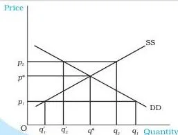
Read Figure 5.1 from the intersection outward. At a price below \( p^* \), demand \( q_1 \) exceeds supply \( q’_1 \), so the gap \( q’_1 q_1 \) is excess demand; some consumers who cannot get the commodity bid the price up, quantity demanded falls, quantity supplied rises, and the market moves back to \( p^* \).
At a price above \( p^* \), supply \( q_2 \) exceeds demand \( q’_2 \) by the gap \( q’_2 q_2 \); firms holding unsold stock lower the price, demand rises and supply falls until the plans match at \( p^* \) (NCERT pp. 72–73).
The Labour Market and Wage Determination
This section reverses the goods-market roles. In the labour market, households are the suppliers of labour and firms are the demanders — the opposite of goods markets. Note that “labour” here means hours of work provided, not the number of labourers (NCERT p. 74).
A profit-maximising firm hires labour up to the point where the extra cost of the last unit of labour equals the extra benefit: the wage equals the marginal revenue product of labour (NCERT p. 75):
\[ w = MRP_L, \qquad MRP_L = MR \times MP_L \]
Because a perfectly competitive firm sells at a fixed price, \( MR = \) price, so the rule becomes \( w = VMP_L \), the value of marginal product of labour — price times marginal product (NCERT p. 75). As long as \( VMP_L \) exceeds the wage, another unit of labour adds profit; if it is below the wage, the firm cuts labour.
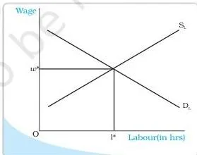
Why the demand curve slopes downward: with diminishing marginal product, a higher wage can be reconciled with \( w = VMP_L \) only by employing less labour — so each firm, and hence the market, demands less labour at higher wages (NCERT p. 75).
On the supply side, each household chooses between income and leisure (NCERT p. 76). A wage rise has two effects: leisure becomes costlier, so the person wants to work more; but income rises, so she can afford more leisure.
At low wages the first effect dominates and labour supply rises with the wage; at high wages the second dominates and supply falls. The result is a backward-bending individual labour supply curve.
The market supply curve, however, stays upward sloping, because higher wages attract many more individuals into the labour force even if some existing workers choose fewer hours (NCERT p. 76). Wage is determined where the downward-sloping demand curve and upward-sloping market supply curve intersect.
Shifts in Demand and Supply: Direction of Change
The single most important distinction in the shift rules: a change in the good’s own price moves us along a curve, while a change in an underlying factor shifts the whole curve (NCERT p. 76).
- Demand shifters: consumer incomes (a normal good like clothes), the number of consumers, tastes, prices of related goods.
- Supply shifters: input prices, technology, the number of firms.
With a fixed number of firms, the four direction rules are (NCERT pp. 77–79):
- Demand shifts right → price rises, quantity rises — e.g. a salary hike shifts the demand for clothes right.
- Demand shifts left → price falls, quantity falls.
- Supply shifts left → price rises, quantity falls — e.g. a rise in input prices raises marginal cost.
- Supply shifts right → price falls, quantity rises — e.g. more firms enter.
A pure demand-side event never moves the supply curve: supply shifts only with changes in the technology or cost conditions of firms, and income or consumer numbers do not affect those (NCERT pp. 77–78). Similarly, an input-price increase does not shift demand, which does not depend on input prices directly (NCERT p. 79).
For demand shifts, price and quantity move in the same direction; for supply shifts, they move in opposite directions.
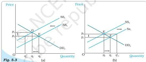
Work through Figure 5.3 panel by panel. In panel (a), supply shifts left to \( SS_2 \) with demand unchanged at \( DD_0 \): at the old price \( p_0 \) there is excess demand, consumers bid the price up, and the new equilibrium G has a higher price \( p_2 \) and lower quantity.
In panel (b), supply shifts right to \( SS_1 \): excess supply at \( p_0 \) makes firms cut price, and the new equilibrium F has a lower price and higher quantity (NCERT p. 78).
Simultaneous Shifts: What Table 5.1 Tells Us
Both curves can move at once, in four combinations. The rule that makes the table memorisable: same direction → quantity certain; opposite direction → price certain. Where the uncertain variable actually lands depends on the magnitudes of the two shifts (NCERT pp. 79–80).

| Shift in demand | Shift in supply | Quantity | Price |
|---|---|---|---|
| Leftward | Leftward | Decreases | May increase, decrease or remain unchanged |
| Rightward | Rightward | Increases | May increase, decrease or remain unchanged |
| Leftward | Rightward | May increase, decrease or remain unchanged | Decreases |
| Rightward | Leftward | May increase, decrease or remain unchanged | Increases |
To see why the table behaves this way, draw a small and then a large shift of one curve while the other shifts by a fixed amount: the intersection moves differently each time, which is exactly why the uncertain variable depends on magnitudes. Figure 5.4 draws two of the four cases and leaves the rest as exercises (NCERT p. 80).
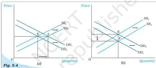
In panel (a), both curves shift right by amounts that balance, so the price is unchanged while quantity rises — if supply had shifted less than demand, the price would have risen. In panel (b), supply shifts right and demand shifts left in balanced amounts, so quantity is unchanged while price falls (NCERT p. 80).
Equilibrium with Free Entry and Exit
This is the second market model, and the key difference is where price comes from. When firms can enter and exit freely, supernormal profit attracts new firms and losses drive firms out, so in equilibrium every firm earns only normal profit and price equals the minimum average cost of the identical firms (NCERT pp. 80–81):
\[ p = \min AC \]
- Price above \( \min AC \) → supernormal profit → new firms enter → supply shifts right → price falls until profit is normal.
- Price below \( \min AC \) → losses → firms exit → supply shifts left → price rises back to the same point.
- At \( p = \min AC \), no firm earns supernormal profit and none incurs a loss, so there is no incentive to enter or exit — this price prevails.
The equilibrium quantity is whatever the market demand curve wants at that price. If each identical firm supplies \( q_{0j} \) at price \( p_0 \), the equilibrium number of firms is (NCERT p. 81):
\[ n_0 = \frac{q_0}{q_{0j}} \]
Example 5.2 shows the reasoning on a wheat market (NCERT p. 82): with free entry and exit, minimum average cost fixes the price, the market demand curve fixes the total quantity at that price, and dividing by each firm’s individual supply gives the number of firms — in the book’s example, six firms.

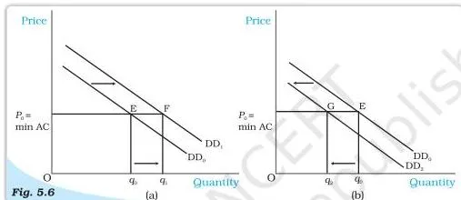
Now trace a demand shift in this model (NCERT pp. 82–83). Demand shifts right: at \( p_0 \) there is excess demand, price tries to rise, supernormal profit attracts new firms, entry shifts supply right, and price returns to \( p_0 \) with a higher quantity \( q_1 \) and more firms \( n_1 \).
Demand shifts left: excess supply makes firms cut price, losses force exit, and price returns to \( p_0 \) with a smaller quantity and fewer firms.
So with free entry and exit, a demand shift changes quantity and the number of firms in the same direction but leaves price unchanged — and the quantity effect is larger than in the fixed-firms case, because entry and exit add to the movement (NCERT p. 83).
Applications: Price Ceiling and Price Floor
The last section applies the demand-supply framework to two government price controls (NCERT p. 84). Watch which limit is set on which side of the market price: a ceiling sits below equilibrium, a floor sits above it.
A price ceiling is the government-imposed upper limit on the price of a good or service. It is generally imposed on necessities — wheat, rice, kerosene, sugar — and is fixed below the market-determined price, because at the market price some sections of the population could not afford these goods (NCERT p. 84).

Work the wheat example through Figure 5.7. The equilibrium price and quantity are \( p^* \) and \( q^* \). The government imposes a ceiling \( p_c \) below \( p^* \); at that price consumers demand \( q_c \) kilograms but firms supply only \( q’_c \), so there is excess demand — a shortage.
The government distributes the limited quantity through a system of rationing: ration coupons restrict how much each person can buy, and the wheat is sold through ration shops, also called fair price shops (NCERT pp. 84–85).
The adverse consequences named in the chapter: consumers must stand in long queues at ration shops, and because rationed quantities leave some people unsatisfied, they are willing to pay more — which may create a black market (NCERT p. 85).
A price floor is the government-imposed lower limit on the price that may be charged. The two classic cases are agricultural price support and minimum wage legislation, both normally set above the market-determined price (NCERT p. 85).
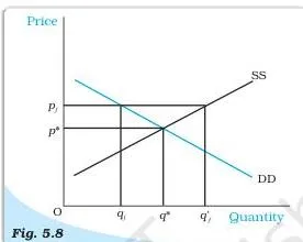
In Figure 5.8, the floor \( p_f \) sits above \( p^* \). At that price firms want to supply \( q’_f \) but the market demands only \( q_f \), so excess supply equal to \( q_f q’_f \) appears. For agricultural support, the government must buy the surplus at the predetermined price to prevent the price from falling (NCERT p. 85).
Edge case to know: a ceiling set above equilibrium, or a floor set below it, would simply not bind — the market price already lies inside the allowed range. That is why the chapter analyses ceilings fixed below, and floors fixed above, the market price.
Reading the Diagrams of Market Equilibrium
Exam answers in this chapter are usually drawn, so know what goes on each graph and where the new equilibrium lands before you write. Work through the figures above in this order, and label every axis, curve and equilibrium point.
- Figure 5.1 (fixed number of firms): axes are price \( P \) and quantity \( Q \); draw \( DD \) downward sloping and \( SS \) upward sloping; label the intersection E, the equilibrium price \( p^* \) and quantity \( q^* \). Mark a price above \( p^* \) and show the excess-supply gap between supply and demand; mark a price below \( p^* \) and show the excess-demand gap. Arrows point toward \( p^* \).
- Labour market diagram: axes are wage \( w \) and labour \( l \); demand for labour slopes downward and is labelled \( w = VMP_L \); the market supply curve slopes upward; their intersection gives the equilibrium wage and employment.
- Figure 5.3 (supply shift): start at E where \( DD_0 \) meets \( SS_0 \); a leftward shift of supply to \( SS_2 \) moves equilibrium up the demand curve to a higher price and lower quantity; a rightward shift to \( SS_1 \) moves it to a lower price and higher quantity.
- Simultaneous shifts: for same-direction movements, fix one curve and draw a small and a large shift of the other; the two possible intersections show why price depends on magnitudes. Label both new equilibria, not just one.
- Figure 5.5 (free entry and exit): draw a horizontal line at \( p_0 = \min AC \); the demand curve cuts it at E; read \( q_0 \) off the quantity axis. There is no upward-sloping \( SS \) line here.
- Figure 5.6: a shifted demand curve cuts the same horizontal price line at a new quantity \( q_1 \) with a new number of firms \( n_1 \); the price stays at \( p_0 \).
- Figure 5.7 (price ceiling): mark \( p^* \) and \( q^* \), draw a dotted horizontal line at the ceiling \( p_c \) below \( p^* \), read off \( q_c \) (demand) and \( q’_c \) (supply) at that price, and shade the gap — it is excess demand, the shortage.
- Figure 5.8 (price floor): draw the dotted line at \( p_f \) above \( p^* \), read \( q’_f \) (supply) and \( q_f \) (demand), and shade the gap — it is excess supply, the surplus.
Chapter 5 Terminology, Explained Simply
A quick-reference glossary in plainer words than the book’s. If you are still stuck on a term, the book’s own glossary appears near the end of the chapter.
| Term | Plain meaning | Where it appears |
|---|---|---|
| Equilibrium | A situation where the plans of all consumers and firms match and the market clears | NCERT p. 71 |
| Equilibrium price \( p^* \) | The price at which market demand equals market supply | NCERT p. 71 |
| Equilibrium quantity \( q^* \) | The quantity bought and sold at the equilibrium price | NCERT p. 71 |
| Excess demand | Quantity demanded exceeds quantity supplied at a price | NCERT p. 71 |
| Excess supply | Quantity supplied exceeds quantity demanded at a price | NCERT p. 71 |
| Invisible hand | The idea that price changes automatically push a market back to equilibrium | NCERT p. 72 |
| Marginal revenue product of labour (\( MRP_L \)) | Marginal revenue times marginal product of labour — the extra benefit of one more unit of labour | NCERT p. 75 |
| Value of marginal product of labour (\( VMP_L \)) | Price times marginal product — equals \( MRP_L \) for a perfectly competitive firm | NCERT p. 75 |
| Normal profit | Profit just enough to cover explicit costs and opportunity costs | NCERT pp. 80–81 |
| Supernormal profit | Profit earned over and above normal profit | NCERT pp. 80–81 |
| Minimum average cost (\( \min AC \)) | The lowest per-unit cost; with free entry and exit, price settles exactly here | NCERT p. 81 |
| Price ceiling | Government-imposed upper limit on the price of a good or service | NCERT p. 84 |
| Price floor | Government-imposed lower limit on the price that may be charged | NCERT p. 85 |
Common Mistakes in Market Equilibrium and Their Fixes
These are the errors this chapter invites, named before you make them. Each row gives the correction and a way to check your own answer.
| Common mistake | Correct rule | How to check your answer |
|---|---|---|
| Calling a change in the good’s own price a “shift” | A price change moves along the curve; income, tastes or the number of consumers shift demand, and input prices, technology or the number of firms shift supply | Ask: what changed? If it is the good’s own price, it is a movement, not a shift |
| Applying the fixed-firms result to the free-entry case | With free entry and exit, a demand shift changes quantity and the number of firms, but never the price | If the question says “free entry and exit”, draw the horizontal \( \min AC \) price line, not an \( SS \) curve |
| Thinking excess demand or excess supply persists | The invisible hand moves price until the market clears; in equilibrium both are zero | Check that your story ends with price at \( p^* \), not stuck at \( p_1 \) |
| Mixing up the simultaneous-shift rows | Same direction → quantity certain; opposite direction → price certain | Write the mnemonic beside the table before answering |
| Assuming a price ceiling always helps consumers | A ceiling below equilibrium creates a shortage — queues, rationing, and possibly a black market | At the ceiling, compare \( q^D \) and \( q^S \); the gap is the shortage |
| Treating the whole labour supply curve as backward bending | Only the individual curve can bend backward; the market curve is upward sloping because higher wages attract more workers | Separate “one individual’s hours” from “all households taken together” |
| Solving for \( p^* \) and forgetting to find \( q^* \) | Always substitute \( p^* \) back into both the demand and supply equations | Verify \( q^D(p^*) = q^S(p^*) \); if the two sides differ, redo the substitution |
Using This Chapter for Exam Practice
This map matches the end-of-chapter exercises to the skill each one tests, so you can practise in the order that builds understanding. Nothing here promises that any particular question will appear.
| Exercises | What they test | What a full answer needs |
|---|---|---|
| 1–4 | Definitions: market equilibrium, excess demand, excess supply; price above and below equilibrium | State the definition (plans match, market clears; compare \( q^D \) and \( q^S \)), then add the adjustment: price rises or falls back to \( p^* \) |
| 5–8 | How price is determined with a fixed number of firms versus free entry and exit; number of firms | Anchor on the \( DD \)-\( SS \) intersection for fixed firms and \( p = \min AC \) for free entry; Q6 runs through supernormal profit → entry → price falls |
| 9–13, 15–16 | Demand and supply shifts, including simultaneous shifts | State the direction rule, then draw a labelled diagram; Q10, Q11 and Q15 expect a full supply-demand graph |
| 14, 21 | Comparison of the fixed-firms and free-entry models | Explain why a demand shift changes quantity more, and price only, when entry and exit are free |
| 17–19 | Labour market: who supplies and demands labour, \( w = MRP_L = VMP_L \), backward-bending supply | Households supply hours of work and firms demand it; wage is set where the curves intersect; Q19 must mention the backward-bending individual supply curve |
| 20, 25 | Applications: price ceiling and price floor reasoning; Q25 is rent control, a ceiling on apartments | Ceiling below market price → shortage; floor above → surplus. Q25: a rent ceiling below the market rent creates excess demand for apartments |
| 22–24 | Numericals mirroring Examples 5.1 and 5.2 | Q22: set \( q^D = q^S \), solve for \( p \), substitute back; Q23: price \( = \min AC \), then quantity from demand and firms \( = q_0 / q_{0j} \); Q24: an input-price rise shifts supply left, a per-unit tax shifts supply again |
A note of caution: textbook contents and the examinable syllabus are not always identical — check the current official syllabus before deciding what to prioritise.
Recap: The Chapter’s Closing Points on Market Equilibrium
These are the ideas the chapter closes with, each compressed to one line for a quick final pass.
- In a perfectly competitive market, equilibrium occurs where market demand equals market supply.
- With a fixed number of firms, the equilibrium price and quantity lie at the intersection of the market demand and market supply curves.
- Each firm hires labour up to the point where the marginal revenue product of labour equals the wage rate.
- Fixed firms, demand shifts right (left): equilibrium price and quantity rise (fall); the supply curve stays put.
- Fixed firms, supply shifts right (left): quantity rises (falls) and price falls (rises); the demand curve stays put.
- When both curves shift in the same direction, the quantity change is certain and the price change depends on magnitudes.
- When they shift in opposite directions, the price change is certain and the quantity change depends on magnitudes.
- With identical firms and free entry and exit, the equilibrium price always equals the minimum average cost of the firms.
- With free entry and exit, a demand shift changes quantity and the number of firms in the same direction but leaves price unchanged; the quantity effect is more pronounced than with a fixed number of firms.
- A price ceiling below equilibrium leads to excess demand; a price floor above equilibrium leads to excess supply.
Related NCERT Class 12 Economics Chapters
The chapters around this one in the same book are its natural next steps. Chapter 4 notes: The Theory of the Firm under Perfect Competition supplies the market supply curve that this chapter draws; Chapter 6, Non-competitive Markets, shows what changes when firms are not price takers, and you can open it from the Class 12 Economics notes page.
For the macroscopic side of the same tools, the Open Economy Macroeconomics notes carry the demand-supply way of thinking into international trade.
If you need the bigger picture first, start from the Class 12 study resource hub or the CBSE notes home to see how this chapter fits your whole subject plan.
Sources and Data Verification
- This page describes the NCERT Class 12 Economics textbook Introductory Microeconomics, Chapter 5 (Market Equilibrium), official edition published on ncert.nic.in.
- The page covers that one book — not Introductory Macroeconomics or Indian Economic Development.
- NCERT settles textbooks, editions and PDFs; CBSE settles curriculum, syllabus and examinations.
- Textbook contents and the examinable syllabus are not always identical — check the current official syllabus for what is examinable.
Frequently Asked Questions: Market Equilibrium Class 12
How do you calculate equilibrium price and quantity in market equilibrium class 12?
Set market demand equal to market supply, solve for the price, then substitute back into either equation. Example: \( q^D = 600 – 2p \) and \( q^S = 300 + p \). Equate: \( 600 – 2p = 300 + p \), so \( 3p = 300 \) and \( p^* = 100 \). Substituting back, \( q^D = 600 – 200 = 400 \) and \( q^S = 300 + 100 = 400 \), so \( q^* = 400 \). The two sides must agree — that agreement is the check that the market clears.
What is the difference between a price ceiling and a price floor?
A price ceiling is a government-imposed upper limit on price, normally set below the market price, which creates excess demand; a price floor is a lower limit, normally set above the market price, which creates excess supply. The chapter’s examples are a ceiling on wheat and floors in agricultural price support and minimum wage legislation (NCERT pp. 84–85).
Why does a shift in demand not change the price when there is free entry and exit?
Because price is pinned at the minimum average cost of the identical firms. A demand increase creates supernormal profit, which attracts new firms; their entry shifts supply right until the price falls back to \( \min AC \). Only the equilibrium quantity and the number of firms rise (NCERT pp. 82–83).
What happens to equilibrium price and quantity when both demand and supply shift to the right?
Quantity certainly increases; price may increase, decrease or remain unchanged depending on the sizes of the shifts. When the two rightward shifts balance exactly, price is unchanged while quantity rises — that is exactly what Figure 5.4(a) draws (NCERT p. 80).
What are the consequences of imposing a price ceiling on a good like wheat?
A shortage: at the ceiling, quantity demanded exceeds quantity supplied. The government rations the limited supply through ration coupons and fair price shops, and the chapter names the adverse consequences — long queues and the possible creation of a black market (NCERT pp. 84–85).
Why is the individual labour supply curve backward bending but the market supply curve not?
An individual trades income against leisure: at high wages the income effect dominates, so she may choose more leisure and supply fewer hours — hence the bend. The market supply curve is built from all households together, and higher wages attract many more people into the labour force, so it slopes upward (NCERT p. 76).
Reference: NCERT Class 12 Economics textbook, chapter 5, official edition on ncert.nic.in.
Explore Class 12 Economics Books
Related chapters: