
Complete revision notes for Class 12 Economics chapter 4, The Theory of the Firm under Perfect Competition, from the rationalised NCERT Introductory Microeconomics textbook. These notes follow the 2026-27 session. The chapter answers one question: how does a firm decide how much to produce?
Its answer — the firm produces the quantity that maximises its profit — is built as a chain of concepts that flow into one another, and this page walks that chain in the same order a good teacher would.
These theory of the firm under perfect competition notes cover the defining features of a perfectly competitive market, the revenue concepts (TR, AR, MR), the three conditions for profit maximisation, the short run and long run supply curves of a firm, what shifts those curves, how individual supply curves combine into the market supply curve, and price elasticity of supply.
The page belongs to our Class 12 Economics notes, within the wider Class 12 and CBSE Notes collections.
How to use this page: first skim the build order below, then read revenue and profit maximisation slowly — every later section depends on them. Revising at the last minute? Start with the One Page Revision Summary, then test yourself with the Key Terms table and the worked examples.
How the Chapter Builds: From Cost Curves to Supply Curves
The previous chapter, Production and Costs, supplied the tool kit — production functions and cost curves. This chapter changes the question: not “how do costs behave?” but “how much should the firm produce?” The textbook assumes the firm is a profit maximiser that sells everything it produces, so output and quantity sold are used interchangeably (NCERT, p. 53).
- Market environment: the four defining features of perfect competition lead to price taking.
- Revenue: total, average and marginal revenue of a price-taking firm.
- Profit maximisation: the three conditions that hold at the best output.
- Firm supply curve: which segment of the marginal cost curve is the supply curve.
- Determinants of supply: technology, input prices and the unit tax.
- Market supply: adding the supply curves of all firms.
- Price elasticity of supply: how supply responds to price.
The chapter’s main results are collected in its closing summary (NCERT, p. 67); the One Page Revision Summary below is built from that list. Once the firm’s supply is clear, the natural next stop is what happens when all firms’ choices meet in the market — covered in our Market Equilibrium notes.
What Makes a Market Perfectly Competitive: Price Taking Behaviour
A market environment has to be fixed before a firm’s profit problem can even be posed. The chapter studies perfect competition, defined by four features (NCERT, p. 53):
- Large number of buyers and sellers — each is tiny compared with the whole market, so no individual can influence the price by size.
- Homogeneous product — the product of one firm cannot be told apart from another’s, so a buyer gets the same good from any firm.
- Free entry and exit — firms can enter or leave easily; this is what keeps the number of firms large.
- Perfect information — all buyers and sellers know the price, quality and other relevant details of the product.
Together these features produce the single most distinguishing characteristic of the market: price taking (NCERT, p. 54). A price-taking firm believes that any price above the market price sells nothing, while at or below the market price it can sell as much as it wants.
Since there is no reason to charge less, a firm that wants to sell sets its price exactly at the market price. The same logic runs from the buyer’s side: a buyer who offers less than the market price finds no seller, while at the market price she can buy any quantity.
Why would a price rise cost the firm every buyer? Because the product is homogeneous and information is perfect — buyers know the prevailing price, switch instantly to the many other firms, and with so many firms no adjustment problem arises (NCERT, p. 54).
Example: a farmer in a large wheat market cannot sell a bag above the going rate; buyers simply move to the next stall. The consequence is that a competitive firm makes exactly one decision — the quantity to produce and sell at the given price.
Revenue in Perfect Competition: TR, AR, MR and the Price Line
A firm earns revenue by selling what it produces. Let \( p \) be the market price of one unit and \( q \) the output the firm sells. Then total revenue (TR) is price multiplied by output (NCERT, p. 54):
\[ TR = p \times q \]
Average revenue (AR) is total revenue per unit of output. Since \( TR = p \times q \), \( AR = TR/q = p \): for a price-taking firm, average revenue equals the market price (NCERT, p. 55). Marginal revenue (MR) is the increase in total revenue from a one-unit increase in output: \( MR = \frac{\Delta TR}{\Delta q} \).
Each extra unit sells at the market price, so the algebra collapses to \( MR = p \). The result worth memorising: for a perfectly competitive firm, \( MR = AR = p \) (NCERT, p. 56).
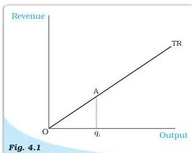
The total revenue curve in Figure 4.1 plots revenue on the vertical axis against output on the horizontal axis. Because \( p \) is constant, the curve is an upward-sloping straight line through the origin — when output is zero, revenue is zero. Its slope, \( Aq_1/Oq_1 \), is exactly the market price (NCERT, p. 55).
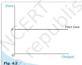
The price line in Figure 4.2 plots the market price against the firm’s output. Since the market price is fixed at \( p \), it is a horizontal straight line at height \( p \).
This line is the firm’s AR curve and also the demand curve facing the firm; it is perfectly elastic, meaning the firm can sell as many units as it wishes at price \( p \) (NCERT, p. 55).
The schedule below uses original numbers at a market price of Rs 25 and shows the three revenue concepts working together:
| Units sold (\( q \)) | TR = 25 \( \times \) \( q \) (in Rs) | MR = change in TR (in Rs) | AR = TR/\( q \) (in Rs) |
|---|---|---|---|
| 0 | 0 | — | — |
| 1 | 25 | 25 | 25 |
| 2 | 50 | 25 | 25 |
| 3 | 75 | 25 | 25 |
| 4 | 100 | 25 | 25 |
| 5 | 125 | 25 | 25 |
At every quantity, AR and MR are both Rs 25 per unit — equal to the market price. Only total revenue grows, in steps of Rs 25, which is exactly why MR stays flat at Rs 25.
Profit Maximisation: The Three Conditions and the Rectangles
Profit (\( \pi \)) is total revenue minus total cost: \( \pi = TR – TC \) (NCERT, p. 56). The firm wants the output \( q_0 \) at which this difference is largest. For a positive profit-maximising output, three conditions must hold at \( q_0 \) (NCERT, p. 56):
- Price equals marginal cost: \( p = MC \). This is the same as \( MR = MC \), because \( MR = p \) for a price taker.
- Marginal cost is non-decreasing at \( q_0 \) — it must not slope downward there.
- Price covers the relevant average cost: in the short run \( p \geq AVC \); in the long run \( p \geq AC \).
Why condition 1: as long as the change in total revenue exceeds the change in total cost, profit keeps rising; once the change in cost overtakes the change in revenue, profit falls. Profit peaks where the two changes are equal — \( MR = MC \), which is \( p = MC \) for the competitive firm (NCERT, p. 56).
Why condition 2: at an output where MC is falling, just left of the intersection MC exceeds price, so a slightly smaller output earns more profit. An intersection on the downward-sloping part of MC is a profit minimum, not a maximum (NCERT, pp. 56-57).
Why condition 3: in the short run, if \( p \lt AVC \), total revenue is less than total variable cost, so the firm loses more than its fixed cost; producing nothing limits the loss to TFC.
In the long run, if \( p \lt AC \), total revenue is less than total cost and the firm makes a loss, whereas shutting down yields zero profit — so it exits (NCERT, pp. 57-58).
Figure 4.3 is the workhorse for conditions 1 and 2. The price line \( p \) cuts the MC curve at several outputs; none of \( q_1 \), \( q_2 \), \( q_3 \), \( q_5 \) and \( q_6 \) can be the maximum.
At \( q_1 \) MC is falling (condition 2 fails); at \( q_2 \) and \( q_3 \) price exceeds MC, so profit is still rising; at \( q_5 \) and \( q_6 \) MC exceeds price, so profit is already falling. Only an intersection on the rising part of MC survives.
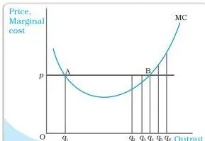
Figure 4.4 shows why the short run needs \( p \geq AVC \). At output \( q_1 \), the price \( p \) is below AVC. TR is the rectangle \( OpAq_1 \) but TVC is the larger rectangle \( OEBq_1 \), so total variable cost exceeds revenue by the area of rectangle \( pEBA \). The firm loses more than its fixed cost, so it produces zero output instead.
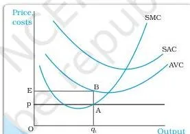
Figure 4.5 repeats the argument for the long run using LRAC. At \( q_1 \) with \( p \) below LRAC, total cost (rectangle \( OEBq_1 \)) exceeds total revenue (rectangle \( OpAq_1 \)) — the firm makes a loss and exits, since shutting down in the long run gives zero profit.
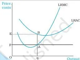
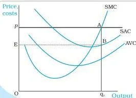
Figure 4.6 puts the three conditions together. The profit-maximising output is \( q_0 \), where the price line meets the rising SMC and \( p \) exceeds AVC. TR is rectangle \( OpAq_0 \), total cost is rectangle \( OEBq_0 \), and profit is the rectangle \( EpAB \) between them.
Memory device — “Match, Rise, Cover”: Match price with marginal cost; make sure marginal cost is Rising (non-decreasing); and price must Cover AVC in the short run or AC in the long run.
Short Run and Long Run Supply Curves: Shut Down and Break Even
A supply schedule lists the quantities a firm chooses to sell at different prices, with technology and factor prices unchanged; the supply curve plots output on the x-axis against price on the y-axis (NCERT, p. 59). The chapter’s central supply result is that a firm’s supply curve is a segment of its marginal cost curve.
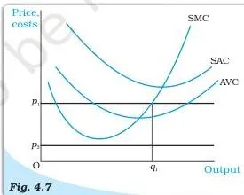
Short run. Two cases decide the shape (NCERT, pp. 59-60). If price \( p_1 \) is at or above minimum AVC, equate \( p_1 \) with SMC on its rising part to get output \( q_1 \); all three profit conditions hold, so the firm supplies \( q_1 \). If price \( p_2 \) is below minimum AVC, then at every positive output AVC exceeds \( p_2 \), and the firm supplies zero.
Figure 4.7 shows both cases on one diagram.
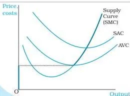
Combining the cases gives the short run supply curve: the rising part of SMC from and above minimum AVC, together with zero output for all prices below minimum AVC. In Figure 4.8, the bold line is that supply curve.
Long run. The same two-case argument with LRMC and LRAC gives: the rising part of LRMC from and above minimum LRAC, plus zero output below it (NCERT, pp. 60-61). Figure 4.9 shows the long run logic for two prices, and Figure 4.10 shows the resulting bold supply curve.
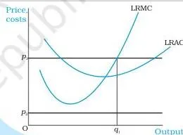
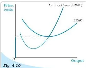
The shut down point is the lowest price at which the firm still produces. In the short run it is the minimum AVC, where the SMC curve cuts the AVC curve; in the long run it is the minimum LRAC (NCERT, p. 61).
Normal profit is the minimum profit needed to keep a firm in its present business; it is part of total cost, best viewed as the opportunity cost of entrepreneurship. Super-normal profit is profit above normal profit.
The break-even point is the point on the supply curve at which the firm earns only normal profit — the minimum of SAC in the short run and of LRAC in the long run (NCERT, p. 61).
Opportunity cost is the gain foregone from the second-best activity (NCERT, p. 61). Example: a student who chooses to study instead of taking a part-time job that pays Rs 5,000 a month gives up that wage; the forgone Rs 5,000 is the opportunity cost of studying.
| Point or curve | Short run | Long run |
|---|---|---|
| Shut down price (below it, output is zero) | minimum AVC | minimum LRAC |
| Break even price (firm earns only normal profit) | minimum SAC | minimum LRAC |
| Supply curve segment | rising part of SMC from and above minimum AVC | rising part of LRMC from and above minimum LRAC |
| Output at the shut down price | positive output at minimum AVC | positive output at minimum LRAC |
Quick way to reconstruct this table: AVC belongs to the short run and AC to the long run; the shut down point sits at the minimum of the relevant average curve, and the break-even point at the minimum of SAC or LRAC.
What Shifts a Firm’s Supply Curve: Technology, Input Prices and Unit Tax
Since the supply curve is a segment of the MC curve, any factor that shifts MC is a determinant of supply (NCERT, p. 62). The chapter works through three:
- Technological or organisational progress — with the same capital and labour, more output is produced, or the same output with fewer inputs. MC falls at every output, so the supply curve shifts right: at any market price the firm supplies more (NCERT, p. 62).
- Rise in input prices — the cost of production rises, raising MC at every output. The supply curve shifts left: at any price the firm supplies less (NCERT, p. 62).
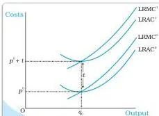
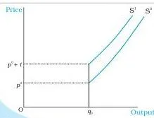
- Unit tax — a fixed amount of tax per unit of output sold. It raises both long run average cost and long run marginal cost by Rs \( t \) at every output, and the long run supply curve shifts left (NCERT, pp. 62-63).
| Change | Effect on MC | Effect on the supply curve |
|---|---|---|
| Technological or organisational progress | MC falls at every output | rightward shift (more supplied at each price) |
| Rise in input prices | MC rises at every output | leftward shift (less supplied at each price) |
| Unit tax of Rs \( t \) | LRAC and LRMC each rise by Rs \( t \) | long run supply shifts left |
Figure 4.11 shows the cost side of the tax: before the tax the firm faces \( LRAC^0 \) and \( LRMC^0 \); after a unit tax of Rs \( t \), every point on both curves is higher by exactly \( t \), giving \( LRAC^1 \) and \( LRMC^1 \). Figure 4.12 shows the supply consequence — the long run supply curve moves from \( S^0 \) to \( S^1 \), a leftward shift.
Market Supply Curve: Adding Firms Horizontally
The market supply curve shows what all firms in the market produce in aggregate at each market price. At any price, it is the sum of the quantities each firm supplies at that price. With \( n \) firms (NCERT, pp. 63-64):
\[ S_m(p) = S_1(p) + S_2(p) + \dots + S_n(p) \]
Geometrically this is a horizontal summation: add quantities across firms at each price — never add prices at a given quantity.
Figure 4.13 builds the market supply curve with two firms that have different cost structures. Firm 1 supplies nothing below price \( \bar{p}_1 \) and firm 2 nothing below \( \bar{p}_2 \), with \( \bar{p}_2 \gt \bar{p}_1 \). Panel (a) shows firm 1’s supply curve \( S_1 \), panel (b) firm 2’s \( S_2 \), and panel (c) the market supply curve \( S_m \).
Below \( \bar{p}_1 \) market supply is zero; between the two minimum prices only firm 1 produces, so the market curve coincides with \( S_1 \); from \( \bar{p}_2 \) upwards both firms produce. At price \( p_3 \), firm 1 supplies \( q_3 \) and firm 2 supplies \( q_4 \), so market supply is \( q_5 = q_3 + q_4 \).
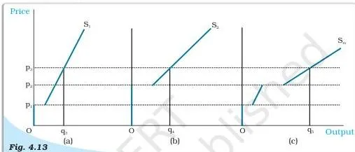
The market supply curve is drawn for a fixed number of firms. If the number of firms increases, market supply shifts right; if it decreases, market supply shifts left (NCERT, p. 64). A worked construction with two firms at different minimum prices is Example C below.
Price Elasticity of Supply: Formula and Geometric Meaning
Price elasticity of supply measures the responsiveness of quantity supplied to a change in price — the percentage change in quantity supplied divided by the percentage change in price (NCERT, p. 65):
\[ e_s = \frac{\text{Percentage change in quantity supplied}}{\text{Percentage change in price}} = \frac{\Delta Q}{Q} \times \frac{P}{\Delta P} \]
Here \( Q \) and \( P \) are the initial quantity and price, and \( \Delta Q \) and \( \Delta P \) are the changes in them. The measure is unit free because the two percentage changes carry no units, and it is positive for an upward-sloping supply curve since quantity and price move together.
A vertical supply curve is completely insensitive to price: \( e_s = 0 \) (NCERT, pp. 65-66).
For straight-line supply curves, the textbook’s Figure 4.14 gives a geometric shortcut. Extend the supply line to meet the quantity axis at \( M \), and take any point \( S \) on the curve with vertical projection \( q_0 \) on the quantity axis. Elasticity at \( S \) is the ratio \( Mq_0/Oq_0 \) (NCERT, p. 66). Three cases follow:
- The line cuts the price axis in its positive range (its extension meets the quantity axis on its negative side at \( M \)): \( Mq_0 \gt Oq_0 \), so \( e_s \gt 1 \).
- The line passes through the origin (\( M \) coincides with \( O \)): \( Mq_0 = Oq_0 \), so \( e_s = 1 \).
- The line cuts the quantity axis on its positive side at \( M \): \( Mq_0 \lt Oq_0 \), so \( e_s \lt 1 \).
Shortcut: intercept on the price axis means elastic supply; a line through the origin means unit elastic supply; an intercept on the quantity axis means inelastic supply.
Key Terms and Definitions at a Glance
One table with the chapter’s full vocabulary — the quick revision anchor, built from NCERT, pp. 53-65.
| Term | Meaning | Example or one-line note |
|---|---|---|
| Perfect competition | Market with many buyers and sellers, homogeneous product, free entry and exit, perfect information | Produces price taking (NCERT, p. 53) |
| Price taking | Firm can sell any quantity at or below the market price, but nothing above it | The firm’s only decision is the quantity to sell |
| Homogeneous product | One firm’s output is identical to every other firm’s | A buyer will not pay more to any one firm |
| Free entry and exit | Firms can enter or leave the market without difficulty | Keeps the number of firms large |
| Perfect information | All buyers and sellers know price, quality and other details | A price rise above the market loses all buyers |
| Total revenue (TR) | Market price \( \times \) quantity sold | \( TR = p \times q \), in rupees |
| Average revenue (AR) | Total revenue per unit of output | \( AR = TR/q = p \) |
| Marginal revenue (MR) | Change in total revenue from one extra unit of output | \( MR = \Delta TR/\Delta q = p \) |
| Price line | Horizontal straight line at the market price | Also the firm’s AR curve and demand curve; perfectly elastic |
| Profit (\( \pi \)) | Total revenue minus total cost | \( \pi = TR – TC \) |
| Normal profit | Minimum profit needed to keep a firm in its business | Treated as part of total cost — the opportunity cost of entrepreneurship |
| Super-normal profit | Profit over and above normal profit | Economic profit beyond covering all costs |
| Shut down point | Lowest price at which the firm still produces | Minimum AVC (short run); minimum LRAC (long run) |
| Break-even point | Point on the supply curve where the firm earns only normal profit | Minimum SAC (short run) or LRAC (long run) |
| Opportunity cost | Gain foregone from the second-best activity | Forgone wage of a student who studies instead of working |
| Supply schedule | Table of quantities a firm sells at different prices, other things unchanged | Technology and factor prices held fixed |
| Supply curve | Graph of the supply schedule | Output on the x-axis, price on the y-axis |
| Market supply curve | Sum of all firms’ supplies at each price | Horizontal summation; shifts right with more firms |
| Price elasticity of supply (\( e_s \)) | Percentage change in quantity supplied per 1% change in price | Unit free; zero for a vertical supply curve |
Formula Sheet: Symbols, Units and How They Fit
All the chapter’s formulas in one table, checked against NCERT, pp. 54-56 and p. 65.
| Formula | Meaning of symbols | Unit or note |
|---|---|---|
| \( TR = p \times q \) | \( p \) = market price (Rs per unit), \( q \) = output sold (units) | TR in rupees |
| \( AR = TR/q = p \) | TR = total revenue, \( q \) = output | Rupees per unit; equals price for a price taker |
| \( MR = \Delta TR/\Delta q = p \) | \( \Delta TR \) = change in total revenue, \( \Delta q \) = change in output | Rupees per unit; equals price for a price taker |
| \( \pi = TR – TC \) | TR = total revenue, TC = total cost | Rupees |
| \( e_s = \frac{\Delta Q}{Q} \times \frac{P}{\Delta P} \) | \( \Delta Q \) = change in quantity supplied, \( Q \) = initial quantity, \( \Delta P \) = change in price, \( P \) = initial price | Unit free; positive for upward-sloping supply, zero for vertical supply |
The one fact to reuse everywhere: for a price-taking firm, \( MR = AR = p \) at every output (NCERT, p. 56). TR and \( \pi \) are measured in rupees; AR and MR in rupees per unit; elasticity has no unit at all. To cross-check any equation or figure against the official text, open the chapter PDF from the NCERT website.
Worked Examples: Solving Numerical Problems Step by Step
Four fully worked problems with original numbers. Learn the method line first, then follow the steps.
Example A: Building a revenue schedule at a market price of Rs 25
Method: for a price taker, \( TR = p \times q \), MR is the change in TR per extra unit, and \( AR = TR/q \).
- Step 1: Fix the market price \( p = 25 \) rupees per unit.
- Step 2: Compute TR for \( q = 0 \) to 5 units using \( TR = 25 \times q \).
- Step 3: MR = change in TR between successive quantities; AR = TR/\( q \).
| \( q \) | TR = 25 \( \times \) \( q \) (in Rs) | MR (in Rs) | AR (in Rs) |
|---|---|---|---|
| 0 | 0 | — | — |
| 1 | 25 | 25 | 25 |
| 2 | 50 | 25 | 25 |
| 3 | 75 | 25 | 25 |
| 4 | 100 | 25 | 25 |
| 5 | 125 | 25 | 25 |
Final answer: \( MR = AR = 25 \) rupees per unit at every quantity — each equals the market price, as required for a price-taking firm.
Example B: Finding the profit-maximising output with price Rs 18
Method: profit at each output is \( \pi = TR – TC \) with \( TR = 18q \); the maximum is where the next unit would add more to cost than to revenue.
- Step 1: Note the fixed cost: \( TFC = TC(0) = 10 \) rupees.
- Step 2: Compute TR and profit at each output.
| \( q \) | TC (in Rs) | TR = 18 \( \times \) \( q \) (in Rs) | \( \pi \) = TR − TC (in Rs) |
|---|---|---|---|
| 0 | 10 | 0 | −10 |
| 1 | 16 | 18 | 2 |
| 2 | 24 | 36 | 12 |
| 3 | 36 | 54 | 18 |
| 4 | 52 | 72 | 20 |
| 5 | 74 | 90 | 16 |
- Step 1: The profit column peaks at \( q = 4 \) with Rs 20 — the unique maximum.
- Step 2: Check the marginal logic: MC from \( q = 3 \) to 4 is \( 52 – 36 = 16 \) rupees (less than 18, so the 4th unit adds profit); MC from \( q = 4 \) to 5 is \( 74 – 52 = 22 \) rupees (more than 18, so the 5th unit would cut profit).
- Step 3: Check the cover condition: at \( q = 4 \), \( AVC = (52 – 10)/4 = 10.5 \) rupees, far below the price of Rs 18.
Final answer: The firm produces 4 units and earns maximum profit of Rs 20; the price of Rs 18 exceeds AVC of Rs 10.5, so all three profit conditions hold.
Example C: Horizontal summation with two firms at different minimum prices
Method: market supply at each price is the sum of the firms’ supplies at that price; a firm contributes zero below its minimum price.
- Step 1: Firm 1 supplies \( S_1(p) = p – 8 \) for \( p \geq 8 \), and zero below 8.
- Step 2: Firm 2 supplies \( S_2(p) = p – 12 \) for \( p \geq 12 \), and zero below 12.
- Step 3: Add the two sources region by region:
\[ S_m(p) = \begin{cases} 0 & : p \lt 8 \ p – 8 & : 8 \leq p \lt 12 \ (p – 8) + (p – 12) = 2p – 20 & : p \geq 12 \end{cases} \]
- Step 1: At \( p = 15 \), \( S_m = 2(15) – 20 = 10 \) units.
- Step 2: Cross-check by firm: firm 1 supplies \( 15 – 8 = 7 \) units and firm 2 supplies \( 15 – 12 = 3 \) units; \( 7 + 3 = 10 \).
Final answer: At the market price of Rs 15, total market supply is 10 units.
Example D: Price elasticity of supply when price rises from Rs 10 to Rs 15
Method: use \( e_s = \frac{\Delta Q}{Q} \times \frac{P}{\Delta P} \) with the initial price and quantity as the base.
Step 1: Initial values: \( P = 10 \) rupees, \( Q = 100 \) units.
New values: \( P_2 = 15 \) rupees, \( Q_2 = 200 \) units.
Step 2: Changes: \( \Delta P = 5 \) rupees, \( \Delta Q = 100 \) units.
\[ e_s = \frac{100}{100} \times \frac{10}{5} = 1 \times 2 = 2 \]
Step 3: Interpretation: quantity supplied rose by 100% while price rose by 50%; the ratio is 2.
Final answer: \( e_s = 2 \), so supply is elastic — quantity supplied responds twice as fast, in percentage terms, as price.
Common Mistakes in Perfect Competition Problems
Seven errors that cost accuracy in numericals and reasoning, each with the correction and a way to check (based on NCERT, pp. 56-66):
| Mistake | Correct rule | How to check your answer |
|---|---|---|
| Confusing the firm’s horizontal demand curve with the market demand curve | The demand curve facing one competitive firm is perfectly elastic (horizontal) at the market price; the market demand curve is downward sloping | Ask whose curve it is: one firm → horizontal; the whole market → downward sloping |
| Using average cost for the short run shut down decision | Short run shut down uses AVC, not AC: produce while \( p \geq AVC \); fixed cost is sunk in the short run | Ask which average is the shut down threshold — short run → AVC |
| Drawing the whole MC curve as the supply curve | Only the rising part of MC from and above minimum AVC (short run) or minimum LRAC (long run) is supply; below that, output is zero | Does your supply curve include the downward-sloping part of MC? If yes, it is wrong |
| Summing supply curves vertically instead of horizontally | Add quantities at each price (horizontal summation), never prices at a given quantity | Pick a price, add each firm’s quantity, and compare with your market curve at that price |
| Treating normal profit as something over and above cost | Normal profit is part of total cost; super-normal profit is what lies over and above cost | If computed profit is zero, the firm still earns normal profit |
| Computing elasticity from the new price and quantity | Use the initial values as the base: \( e_s = \frac{\Delta Q}{Q} \times \frac{P}{\Delta P} \) | Recompute with initial \( P \) and \( Q \), not the new values |
| Thinking a profit-maximising firm can produce where MC is falling | At a downward-sloping MC intersection profit is a minimum, not a maximum; MC must be non-decreasing | At your chosen output, is MC rising? If not, the output is not profit maximising |
Misconception Autopsy: Why Minimum Average Cost Is Not the Target
Students often conclude that a profit-maximising firm should produce at the output where average cost is lowest. That output indeed minimises cost per unit, but it has no direct link to profit. Profit is total revenue minus total cost, so what matters is the last unit: does it add more to revenue than to cost?
That question is answered by the equality \( p = MC \) with MC rising, and with price covering AVC or AC. A low average cost matters only indirectly, as one ingredient of the profit rectangle in Figure 4.6. The output rule is price equals marginal cost — never “produce where AC is minimised” (NCERT, pp. 56-58).
How to Write Complete Answers to the Textbook Exercises
The chapter’s exercises (NCERT, pp. 67-70) fall into three groups, and each group needs its own answer structure:
| Type of question | Exercise numbers | What a complete answer must include |
|---|---|---|
| Definition / direct concept | 1, 2, 3, 5, 6, 7, 12, 13, 14, 15, 16, 17, 18 | Open with the definition, then state the consequence or relation. For the conditions in exercise 7, list all three and separate the short run (\( p \geq AVC \)) from the long run (\( p \geq LRAC \)) cases. |
| Reasoning (why, can there be, will a firm ever) | 4, 8, 9, 10, 11 | Verdict first (“No, because …”), then argue from the three profit conditions: compare MR with MC, check the slope of MC, and compare \( p \) with AVC or AC. An intersection on falling MC is a minimum, so it cannot maximise profit. |
| Numericals | 19, 20, 21, 22, 23, 24, 25, 26, 27 | Formula → substitution → result with units → one-line conclusion. For elasticity questions, base each percentage on the initial values. |
For any supply curve question, name the exact segment you are describing: the rising part of SMC from and above minimum AVC (short run) or the rising part of LRMC from and above minimum LRAC (long run), with zero output below the shut down price.
Where the question asks for a diagram, sketch the labelled curve and name it — the price line, the short run supply curve, the long run supply curve, or the market supply curve — so the answer is self-contained.
One Page Revision Summary
Everything the chapter’s closing summary establishes (NCERT, p. 67), compressed into one list:
- Price taking: firms in perfect competition take the market price as given.
- Revenue: \( TR = p \times q \); for a price taker \( AR = p \) and \( MR = p \).
- Demand facing the firm: perfectly elastic — a horizontal line at the market price.
- Profit: \( \pi = TR – TC \).
- Short run conditions: \( p = SMC \); SMC non-decreasing; \( p \geq AVC \).
- Long run conditions: \( p = LRMC \); LRMC non-decreasing; \( p \geq LRAC \).
- Short run supply: rising part of SMC from and above minimum AVC, plus zero output below.
- Long run supply: rising part of LRMC from and above minimum LRAC, plus zero output below.
- Shifts: technological progress shifts supply right; higher input prices shift it left; a unit tax shifts it left.
- Market supply: horizontal summation of individual supply curves; more firms shift it right, fewer shift it left.
- Elasticity: \( e_s = \frac{\Delta Q}{Q} \times \frac{P}{\Delta P} \); unit free; \( e_s = 0 \) for a vertical supply curve.
Frequently Asked Questions on the Theory of the Firm
Why is the demand curve facing a perfectly competitive firm perfectly elastic?
Because the firm is a price taker. With many firms selling an identical product and perfect information, the firm can sell any quantity at the market price but nothing above it.
A horizontal straight line at the market price — the price line — is exactly that situation, and perfectly elastic demand means the firm faces no quantity limit at that price (NCERT, p. 55).
What is the difference between the shut down point and the break even point?
The shut down point is the lowest price at which the firm still produces: minimum AVC in the short run and minimum LRAC in the long run. The break-even point is where the firm earns only normal profit: the minimum of SAC (short run) or LRAC (long run).
Below the shut down price the firm produces zero output; at the break-even price it covers all costs, including normal profit (NCERT, p. 61).
Why will a firm produce in the short run when price is below average cost but above average variable cost?
Because fixed costs are already committed in the short run. When \( p \gt AVC \), every unit sold contributes more than its variable cost, so the loss is smaller than the fixed cost the firm must pay anyway.
Only when \( p \lt AVC \) does producing make the loss larger than TFC; then zero output is better, and the firm shuts down (NCERT, pp. 57-58).
Why is normal profit treated as part of total cost?
Normal profit is the minimum return that keeps the entrepreneur in this business — the opportunity cost of entrepreneurship, the gain foregone from the next best use of the entrepreneur’s time and money. Since total cost must include every cost of staying in business, normal profit is counted inside total cost (NCERT, p. 61).
How do you build the market supply curve when firms start supplying at different minimum prices?
Add the firms’ supplies at each price — a horizontal summation. Below the lower minimum price, market supply is zero; between the two minimum prices, only the cheaper firm produces; from the higher minimum price upwards, both produce.
This is exactly what Example C does: firm 1 starts at price 8 and firm 2 at price 12, giving market supply of zero below 8, \( p – 8 \) between 8 and 12, and \( 2p – 20 \) from 12 upwards.
How do you read the geometric method for price elasticity of supply?
Extend the straight-line supply curve to meet the quantity axis at \( M \); take a point \( S \) on the curve with vertical projection \( q_0 \) on the quantity axis. Elasticity at \( S \) is \( Mq_0/Oq_0 \).
A supply line that cuts the price axis gives \( e_s \gt 1 \); one through the origin gives \( e_s = 1 \); one that cuts the quantity axis on its positive side gives \( e_s \lt 1 \) (NCERT, p. 66).
Reference: NCERT Class 12 Introductory Microeconomics textbook, chapter 4.
Explore Class 12 Economics Notes
- Class 12 Economics Notes
- Class 12 CBSE Notes
- CBSE Notes for Classes 1 to 12
- Previous: Production and Costs
- Next: Market Equilibrium
Class 12 Economics on LearnCBSE:
Related chapters:
- A Simple Economy notes
- Theory of Consumer Behaviour notes