
These are the complete revision notes for Theory of Consumer Behaviour, Chapter 2 of the NCERT Class 12 Introductory Microeconomics textbook (the chapter covers NCERT pp. 8–35). The page condenses the entire chapter — utility, indifference curves, the budget line, demand and elasticity — into compact definitions, tables, formulas, diagrams and solved examples, so you can revise it quickly and completely.
These notes follow the 2026-27 session.
The chapter studies one question: how does a consumer choose the best combination of goods she can afford? Economists call this the problem of choice, and the chapter answers it in two ways — cardinal utility analysis and ordinal utility analysis. Both lead to the same destination, a downward-sloping demand curve, through different routes.
Read the sections top to bottom, or jump straight to the part you need from the contents below.
Reference: NCERT Class 12 Introductory Microeconomics textbook, chapter Theory of Consumer Behaviour. The official textbook is available for free download from the NCERT website; the page references below (NCERT, p. X) point to that edition.
The Consumer’s Problem: Two Ways Economics Explains Choice
Economics opens this chapter with a single question: how should a consumer spend a limited income on different goods to get the maximum satisfaction? Economists call this the problem of choice (NCERT, p. 8). The ‘best’ combination depends on two things — the consumer’s preferences (her likes) and what she can afford, which depends on the prices of goods and her income.
To keep the analysis simple, the chapter assumes only two goods: bananas (good 1, quantity \( x_1 \)) and mangoes (good 2, quantity \( x_2 \)). Any combination \( (x_1, x_2) \) is called a consumption bundle, or simply a bundle (NCERT, p. 8).
The central idea the whole chapter builds on is utility — the want-satisfying capacity of a commodity. The stronger the desire for a commodity, the greater its utility.
Utility is subjective: a chocolate lover gets far more utility from a chocolate than someone indifferent to it, and a room heater yields more utility in Ladakh than in Chennai, and more in winter than in summer (NCERT, pp. 8–9).
Because utility is subjective, economists have developed two ways of studying choice:
- Cardinal utility analysis assumes utility can be expressed in numbers — “this shirt gives me 50 units of utility.”
- Ordinal utility analysis assumes the consumer can only rank bundles — “I prefer bundle A to bundle B” — without measuring how much more she likes A.
| Basis | Cardinal utility analysis | Ordinal utility analysis |
|---|---|---|
| Measurement of utility | Expressed in numbers (units of utility) | Only ranked, not measured |
| What the consumer can say | “This bundle gives 50 units of utility” | “Bundle A is preferred to bundle B” |
| Main tools | Total utility, marginal utility, law of diminishing MU | Indifference curves and the budget line |
| Why demand slopes down | Diminishing marginal utility | Tangency of an indifference curve with the budget line |
Cardinal Utility: Total Utility, Marginal Utility and the Demand Curve
Total utility (TU) of a commodity is the total satisfaction a consumer gets from consuming a given quantity of it. TU depends on the quantity consumed, so \( TU_n \) means the total utility from \( n \) units. Marginal utility (MU) is the change in total utility caused by consuming one additional unit (NCERT, p. 9):
\[ MU_n = TU_n – TU_{n-1} \]
Working the other way, total utility is the sum of the marginal utilities of all the units consumed (NCERT, p. 9):
\[ TU_n = MU_1 + MU_2 + \dots + MU_n \]
The relationship follows the law of diminishing marginal utility: as consumption of a commodity increases (other consumption held constant), the marginal utility from each additional unit declines. Why? Once a consumer has some amount of the commodity, her desire for still more becomes weaker (NCERT, pp. 9–10).
Notice the pattern this creates: TU rises but at a diminishing rate; when TU is constant, MU is zero; once TU falls, MU turns negative (NCERT, p. 10).
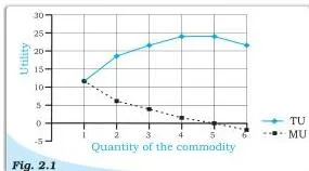
Figure 2.1 shows the same story in pictures: total utility climbs while marginal utility slides down; where TU flattens, MU touches zero; where TU starts falling, MU is negative. This steady decline is the law of diminishing marginal utility at work.
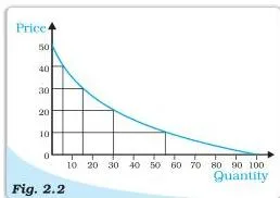
This single law explains the downward-sloping demand curve. A consumer who buys some quantity of a commodity at a given price values each further unit less than the previous one, so she will buy the next unit only if the price drops.
The demand curve in Figure 2.2 therefore slopes downward: at lower prices the consumer buys more; at higher prices she buys less (NCERT, pp. 10–11). This negative price-quantity relationship is the law of demand.
From Preferences to Indifference Curves
Cardinal analysis fails in one obvious way: in real life nobody measures satisfaction in numbers. What people actually do is rank the bundles available to them (NCERT, p. 11). This is the starting point of the ordinal approach.
Take all the bundles that give the consumer equal satisfaction and join them into a curve. That curve is an indifference curve (IC) — a curve joining all bundles among which the consumer is indifferent (NCERT, p. 11). Figure 2.3 shows one such curve with bundles A, B, C and D, all giving the same level of satisfaction.
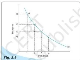
Moving along the curve, when the consumer gains one more banana she must give up some mangoes to stay at the same satisfaction. This trade-off is measured by the marginal rate of substitution (MRS) — the amount of mangoes foregone to get one additional banana while total utility stays constant. Formally (NCERT, p. 11):
\[ MRS = \left| \frac{\Delta Y}{\Delta X} \right| \]
The absolute-value bars matter: if \( \Delta Y / \Delta X = -3/1 \), then MRS = 3 (NCERT, p. 11).
Now watch what happens as the consumer gets more bananas. The law of diminishing marginal rate of substitution says the MRS falls as bananas increase. The reason is the same process we met before: as bananas accumulate, their marginal utility falls, while the shrinking stock of mangoes makes their marginal utility rise.
So the consumer sacrifices smaller and smaller amounts of mangoes for each extra banana (NCERT, p. 12). In Figure 2.3, moving from A to B means giving up 3 mangoes for 1 banana, from B to C only 2, and from C to D just 1.
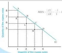
This diminishing MRS is what makes an indifference curve convex to the origin — the usual shape. There is one exception: for perfect substitutes, MRS does not diminish; it stays constant. Figure 2.4 shows five-rupee notes and five-rupee coins — for the consumer both are just “five rupees”, so she will always trade one coin for one note without changing satisfaction.
The indifference curve is a straight line (NCERT, pp. 12–13).
Two more ideas complete the preference framework. Monotonic preferences assume that between any two bundles, the consumer prefers the one that has more of at least one good and no less of the other good (NCERT, p. 13).
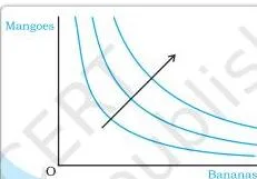
And the full collection of a consumer’s indifference curves is her indifference map; because of monotonicity, bundles on higher indifference curves are preferred to bundles on lower ones (NCERT, p. 13).
Three Properties of Indifference Curves You Must Be Able to Prove
Three properties of indifference curves follow directly from monotonic preferences. They are standard theory answers, so be ready to state each one and explain why it holds.
Property 1: Indifference curves slope downwards from left to right
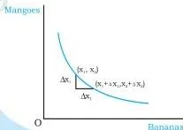
To have more bananas on the same curve, the consumer must forego some mangoes. If she could get more bananas without giving up mangoes, she would have more of at least one good and no less of the other — a bundle on a higher curve.
Since she stays on the same curve, an increase in bananas must be compensated by a decrease in mangoes: if \( \Delta x_1 \gt 0 \), then \( \Delta x_2 \lt 0 \) (NCERT, p. 13). Figure 2.6 shows exactly this.
Property 2: A higher indifference curve gives greater utility
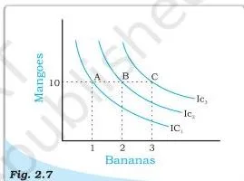
As long as marginal utility is positive, more of a commodity increases satisfaction (NCERT, p. 14). Consider bundles A (1 banana, 10 mangoes), B (2 bananas, 10 mangoes) and C (3 bananas, 10 mangoes) — mangoes are fixed, bananas increase. Since B has more bananas than A, B lies on a higher curve than A; similarly C lies higher than B.
More of either good pushes the bundle to a higher indifference curve, as Figure 2.7 illustrates.
Property 3: Two indifference curves never intersect
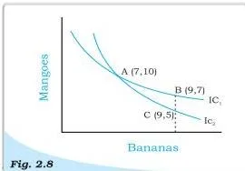
Suppose they did, as in Figure 2.8. Let A and B lie on curve IC₁ and A and C on curve IC₂. Since A and B are on the same curve, they give equal utility; since A and C are on the same curve, they also give equal utility. It would then follow that B and C give equal utility too.
But B contains the same quantity of bananas as C and more mangoes — so B must be strictly preferred to C. Equal and unequal at the same time is a contradiction, so intersection is impossible (NCERT, pp. 14–15).
| Property | Statement | Why it holds |
|---|---|---|
| 1 | Indifference curves slope downward | More of one good on the same curve must be offset by less of the other |
| 2 | Higher curve = higher utility | Marginal utility is positive, so more of any good raises satisfaction |
| 3 | Indifference curves never intersect | Intersection would make a strictly preferred bundle equal in utility to itself — contradiction |
Budget Set and Budget Line: The Consumer’s Affordable Bundles
Preferences tell us what the consumer likes; the budget tells us what she can get. With income \( M \) and prices \( p_1 \) (bananas) and \( p_2 \) (mangoes), spending on a bundle \( (x_1, x_2) \) is \( p_1x_1 + p_2x_2 \) (NCERT, p. 15).
- Budget constraint: the consumer can buy any bundle that costs no more than her income — \( p_1x_1 + p_2x_2 \leq M \) (NCERT, p. 15).
- Budget set: the collection of all bundles she can afford at the prevailing prices — all bundles satisfying the constraint.
- Budget line: the bundles that cost exactly her entire income — \( p_1x_1 + p_2x_2 = M \) (NCERT, p. 16).
Rewriting the budget line in slope-intercept form gives (NCERT, p. 16):
\[ x_2 = \frac{M}{p_2} – \frac{p_1}{p_2}x_1 \]
From this form we can read everything at a glance:
- Horizontal intercept \( M/p_1 \) — the bananas she can buy by spending all income on bananas;
- Vertical intercept \( M/p_2 \) — the mangoes she can buy by spending all income on mangoes;
- Slope \( -p_1/p_2 \) — the price ratio.
Why is the slope the price ratio? Take two points on the budget line. Since both cost exactly \( M \), the increased spending on bananas must be exactly offset by reduced spending on mangoes: \( p_1\Delta x_1 + p_2\Delta x_2 = 0 \), which rearranges to \( \Delta x_2/\Delta x_1 = -p_1/p_2 \) (NCERT, p. 17).
In words, the price ratio tells us the rate at which the market lets the consumer trade mangoes for bananas: to gain one more banana she must give up \( p_1/p_2 \) mangoes (NCERT, p. 16).
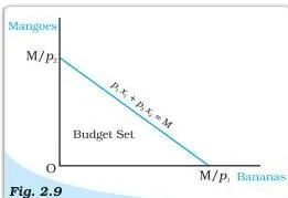
Figure 2.9 draws this: bananas on the horizontal axis, mangoes on the vertical axis, and the budget set is everything on or below the line. Points below the line cost strictly less than \( M \); points above it are unaffordable (NCERT, p. 16).
Income Changes Shift; Price Changes Pivot: Movements of the Budget Line
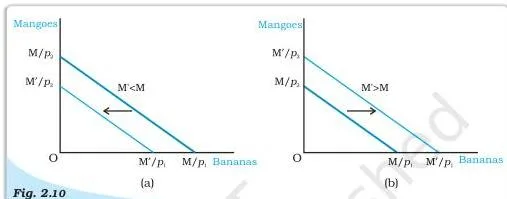
The budget set changes whenever income or either price changes. The kind of change tells us which variable moved (NCERT, pp. 17–18):
- Income change: both intercepts change but the slope stays the same, so the budget line shifts parallel — outward when income rises, inward when income falls. Figure 2.10 shows the inward shift in panel (a) and the outward shift in panel (b).
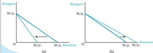
- Change in one price: the intercept of the good whose price did not change stays fixed, while the slope and the other intercept change. If the price of bananas rises, the line becomes steeper and pivots inwards; if it falls, the line becomes flatter and pivots outwards. Figure 2.11 shows the steeper line in panel (a) and the flatter one in panel (b).
| Cause | Horizontal intercept \( M/p_1 \) | Vertical intercept \( M/p_2 \) | Slope \( -p_1/p_2 \) | Movement |
|---|---|---|---|---|
| Income rises | Increases | Increases | Unchanged | Parallel outward shift |
| Income falls | Decreases | Decreases | Unchanged | Parallel inward shift |
| Price of good 1 rises | Decreases | Unchanged | Becomes steeper (more negative) | Pivot inward around the vertical intercept |
| Price of good 1 falls | Increases | Unchanged | Becomes flatter (less negative) | Pivot outward around the vertical intercept |
The Consumer’s Optimum: Where Budget Line Touches the Highest Indifference Curve
A rational consumer knows her preferences and always chooses the bundle that gives maximum satisfaction from the set of bundles she can afford (NCERT, p. 20). So her problem is simple: reach the highest possible indifference curve while staying within her budget set.
Two location rules decide the answer (NCERT, p. 20):
- The optimum lies on the budget line. A point below the line can never be optimal, because monotonicity guarantees that some point on the line has more of at least one good and no less of the other. Points above the line are unaffordable.
- On the budget line, the optimum is the point where the line is tangent to an indifference curve — the point where it just touches the highest curve reachable. Every other point on the budget line lies on a lower indifference curve, so it is inferior.
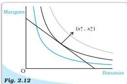
Read Figure 2.12 carefully. The indifference curve that just touches the budget line is the highest possible curve given the budget set. The grey curve above it is not affordable; the blue curve below it is inferior to the touching curve; and any other point on the budget line sits on a lower curve than the touching one.
The optimum is the tangency point \( (x_1^*, x_2^*) \) (NCERT, p. 20).
At tangency the slopes are equal in absolute value — the slope of the indifference curve is the MRS and the slope of the budget line is the price ratio (NCERT, p. 19):
\[ MRS = \frac{p_1}{p_2} \]
This equality has a clean interpretation: at the optimum, the rate at which the consumer is willing to substitute bananas for mangoes (MRS) equals the rate at which the market lets her substitute them (the price ratio).
Suppose MRS were 3 while the price ratio were 2: the consumer would willingly give up 3 mangoes for one banana, but the market demands only 2, so buying the banana leaves her with more of both goods — a strictly preferred bundle. The same argument rules out any point where MRS differs from the price ratio (NCERT, p. 19).
One exception: the tangency story assumes the optimum is an interior point. In some situations the optimum lies at a corner, where the consumer spends her entire income on only one of the goods (NCERT, footnote 9, pp. 20–21).
Demand, the Demand Curve and the Law of Demand
Demand for a commodity is the quantity a consumer is willing to buy and able to afford, given the prices of goods, her income and her tastes (NCERT, p. 21). Keeping everything except own price fixed, the amount optimally chosen becomes a function of the price alone — the demand function, written as (NCERT, p. 23):
\[ X = f(P) \]
A quick note on functions: a function \( y = f(x) \) assigns exactly one value of \( y \) to each value of \( x \); it is increasing if \( y \) does not decrease as \( x \) rises, and decreasing if \( y \) does not increase as \( x \) rises (NCERT, pp. 21–22). Demand is a decreasing function of price.
The graph of the demand function is the demand curve (NCERT, p. 23). Economics uses an unusual convention here: the independent variable (price) is measured on the vertical axis and the dependent variable (quantity) on the horizontal axis — the opposite of what mathematics usually does (NCERT, p. 22). Figure 2.13 shows the result.
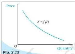
The negative slope of the demand curve is the law of demand: other things being equal, the quantity demanded of a commodity and its price are negatively related — demand falls when price rises and rises when price falls (NCERT, p. 24).
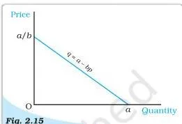
A particularly useful form is the linear demand function (NCERT, p. 24):
\[ d(p) = a – bp \quad \text{for } 0 \leq p \leq \frac{a}{b}, \qquad d(p) = 0 \quad \text{for } p \gt \frac{a}{b} \]
Here \( a \) is the vertical intercept (quantity demanded when price is zero), \( -b \) is the slope (a one-unit rise in price cuts demand by \( b \) units), and \( a/b \) is the price at which demand falls to zero. Figure 2.15 draws this line.
How the Demand Curve Is Derived and Why It Slopes Downward
The demand curve is not an assumption — it can be derived from the indifference-curve and budget-line model. The textbook’s Figure 2.14 shows the two-panel derivation; its logic runs like this (NCERT, p. 23):
- First point: with banana price \( P’_1 \), mango price \( P’_2 \) and income \( M \), the consumer’s optimum is at point C, where she buys \( X’_1 \) bananas and \( X’_2 \) mangoes. Plot \( P’_1 \) against \( X’_1 \) in a second diagram — that is the first point on the demand curve.
- Price falls: drop the price of bananas to \( \bar{P}_1 \), keeping \( P’_2 \) and \( M \) constant. The budget set expands, the new optimum D lies on a higher indifference curve, and she buys more bananas (\( \bar{X}_1 \gt X’_1 \)). Plot \( \bar{P}_1 \) against \( \bar{X}_1 \) — the second point.
- Repeat: another price fall gives a third point. Joining all the price-quantity pairs traces the demand curve, which slopes downward because each price fall raised quantity demanded.
Why does the new optimum always involve more bananas at a lower price? Two effects work together (NCERT, pp. 23–24):
- Substitution effect: bananas have become relatively cheaper, so the consumer substitutes bananas for mangoes in order to maintain her satisfaction.
- Income effect: the price fall raises her real purchasing power — she can buy the same bundle as before and still have money left over — and this further raises her demand for bananas (and other goods).
Both effects push quantity demanded in the same direction when price changes, which is why the demand curve is generally downward sloping.
Normal Goods, Inferior Goods, Substitutes and Complements
So far price was the changing variable. The same demand framework also classifies goods by how demand responds to income and to the prices of related goods:
- Normal goods: the quantity demanded moves in the same direction as income — income rises, demand rises (NCERT, p. 24).
- Inferior goods: the quantity demanded moves in the opposite direction to income — income rises, demand falls. The textbook’s example is coarse cereals (NCERT, pp. 24–25).
- Substitutes: goods used in place of each other. Demand for a good moves in the same direction as the price of its substitute — if coffee becomes costlier, tea is consumed more (NCERT, p. 25).
- Complements: goods consumed together. Demand for a good moves in the opposite direction to the price of its complement — if sugar becomes costlier, tea consumption falls (NCERT, p. 25).
Two qualifications from the chapter are worth remembering:
- A good can change its category with income. At very low incomes, demand for low-quality cereals rises with income; beyond some income level, further income growth makes the consumer switch to better-quality cereals, so the same good becomes inferior (NCERT, p. 25).
- Giffen good exception. For some goods, the income effect is so strong that it outweighs the substitution effect; demand then responds positively to the good’s own price. Such a good is called a Giffen good (NCERT, p. 24).
| Type of good | Demand as income rises | Demand when the related good’s price rises | Textbook example |
|---|---|---|---|
| Normal | Rises | — | Most goods |
| Inferior | Falls | — | Coarse cereals |
| Substitute | — | Rises (same direction) | Tea and coffee |
| Complement | — | Falls (opposite direction) | Tea and sugar |
Movement along the Demand Curve versus Shifts of the Demand Curve
The demand curve is drawn with income, prices of other goods and preferences held fixed. A change in the good’s own price moves the consumer along the curve; a change in any of the other determinants shifts the whole curve (NCERT, p. 26).
Figure 2.17 contrasts the two cases: panel (a) is a movement along the curve, panel (b) a shift of the curve.
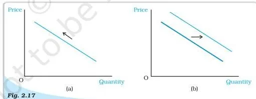
Figure 2.16 shows the two directions of a shift — leftward in panel (a) and rightward in panel (b). Shifts always come from a change in some factor other than the good’s own price (NCERT, p. 26).
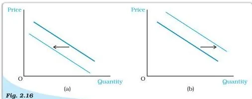
The table below collects the standard cases (NCERT, pp. 25–26):
| Change | Effect on the demand curve |
|---|---|
| Price of the good itself falls | Movement down along the curve |
| Income rises (normal good) | Shift rightward |
| Income rises (inferior good) | Shift leftward |
| Price of a substitute rises | Shift rightward |
| Price of a complement rises | Shift leftward |
| Preferences change in favour of the good | Shift rightward |
| Preferences change against the good | Shift leftward |
Market Demand: Horizontal Summation of Individual Demand Curves
Individual demand is one consumer’s choice; market demand is the demand of all consumers taken together. At any price, market demand is the sum of the quantities demanded by every consumer at that price (NCERT, p. 27).
Graphically, the market demand curve is obtained by adding the individual demand curves horizontally — at each price, add the quantities demanded, as Figure 2.18 shows (NCERT, p. 27).
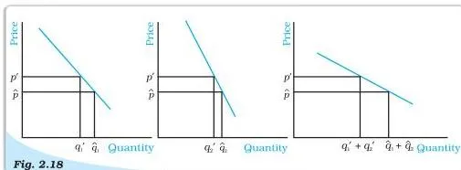
One detail matters when using formulas: a consumer’s demand is zero above her maximum price. So when adding two demand functions, add them only in the price range where both are positive; in higher ranges the market demand equals the demand of whichever consumer is still buying. The result is a piecewise market demand function (NCERT, p. 27).
A complete numerical example with the functions \( d_1(p) = 12 – p \) and \( d_2(p) = 18 – 2p \) is worked out below.
Price Elasticity of Demand: Definition, Formula and Classification
Price elasticity of demand measures how responsive the quantity demanded of a good is to changes in its price (NCERT, p. 28). It is defined as the percentage change in demand divided by the percentage change in price:
\[ e_D = \frac{\text{percentage change in demand}}{\text{percentage change in price}} = \frac{\frac{\Delta Q}{Q} \times 100}{\frac{\Delta P}{P} \times 100} = \frac{\Delta Q/Q}{\Delta P/P} \]
where \( \Delta P \) is the change in price and \( \Delta Q \) is the change in quantity (NCERT, p. 28). Since price and quantity move in opposite directions, \( e_D \) comes out negative; the chapter therefore always works with the absolute value \( |e_D| \) (NCERT, p. 28).
Elasticity is also a pure number — the percentage changes cancel all units, so it carries no rupees, kilograms or any other unit (NCERT, p. 34).
Comparing the two percentage changes classifies demand (NCERT, pp. 28–29):
| Value of \( |e_D| \) | Name | Meaning | Typical goods |
|---|---|---|---|
| \( \lt 1 \) | Inelastic | Quantity changes proportionally less than price | Essentials |
| \( = 1 \) | Unitary elastic | Quantity changes proportionally the same as price | — |
| \( \gt 1 \) | Elastic | Quantity changes proportionally more than price | Luxuries |
Elasticity Along a Linear Demand Curve: Formula, Geometric Measure and Special Cases
On a straight-line demand curve \( q = a – bp \), each one-unit price change changes quantity by \( -b \). Substituting into the elasticity formula gives elasticity at price \( p \) as (NCERT, p. 29):
\[ e_D = -\frac{bp}{a – bp} \]
This single formula shows that elasticity is different at every point of a linear demand curve (NCERT, p. 29):
- At \( p = 0 \) (the horizontal intercept), \( e_D = 0 \).
- At \( q = 0 \) (the vertical intercept), \( e_D = \infty \).
- At the midpoint \( p = a/2b \), \( e_D = 1 \).
- Above the midpoint (higher price), \( e_D \gt 1 \); below the midpoint, \( e_D \lt 1 \).
Figure 2.19 marks these values along the line.
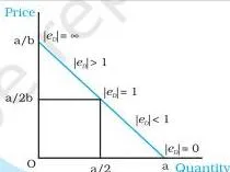
Memory hook — “middle means one”: at the midpoint of a straight-line demand curve elasticity is exactly 1; every point above the midpoint is elastic (elasticity greater than 1) and every point below it is inelastic (less than 1). That one fact lets you locate the elastic, unitary and inelastic zones on any straight demand curve instantly.
Geometric measure. Because elasticity involves ratios, it can be read straight off the diagram: at any point on a straight-line demand curve, \[ e_D = \frac{\text{lower segment}}{\text{upper segment}} \]
The rule works because the small triangles formed by the price line and the demand curve are similar, so the ratio of the two segments equals the ratio of the percentage changes that defines elasticity (NCERT, p. 30).
The same conclusions follow: elasticity is 0 where the curve meets the horizontal axis, infinite where it meets the vertical axis, and 1 at the midpoint.
Constant elasticity demand curves. Some demand curves have the same elasticity at every point (NCERT, pp. 30–31). Figure 2.20 shows the three standard cases:
- Panel (a), a vertical demand curve: whatever the price, quantity stays at \( \bar{q} \), so \( |e_D| = 0 \) — perfectly inelastic.
- Panel (b), a horizontal demand curve: the price stays at \( \bar{P} \) whatever the quantity, and any different price drops demand to zero, so \( |e_D| = \infty \) — perfectly elastic.
- Panel (c), a rectangular hyperbola: a percentage change in price always produces an equal percentage change in quantity, so \( |e_D| = 1 \) at every point — unitary elastic.
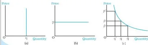
Read Figure 2.20 panel by panel.
The vertical curve says “no quantity change, whatever the price”; the horizontal curve says “no price change, whatever the quantity”; the rectangular hyperbola says “price times quantity is constant everywhere” — a curve of the form \( xy = c \), which for demand means \( pq = c \), so total expenditure \( p \times q \) is the same at every point (NCERT, p. 32).
What Determines Elasticity? And How It Affects Consumer Expenditure
Two factors mainly decide how elastic demand for a good is (NCERT, p. 31):
- Nature of the good: necessities such as food are price inelastic — people keep buying food even when it gets dearer. Luxuries are price elastic.
- Availability of close substitutes: when close substitutes are easily available, demand is elastic (consumers can switch); when they are not, demand is inelastic. The textbook’s example: a particular variety of pulses has more elastic demand than food as a whole, because buyers can switch to another variety (NCERT, p. 31).
Elasticity and expenditure. Expenditure on a good is \( \text{price} \times \text{quantity} \). Since price and quantity move in opposite directions, whether spending rises or falls after a price change depends on which percentage change is bigger (NCERT, pp. 31–32). The six cases from the chapter’s Table 2.5:
| Price change | % change in price | % change in quantity | Effect on expenditure | Elasticity |
|---|---|---|---|---|
| Rise | +10 | −8 | Rises | Inelastic |
| Rise | +10 | −12 | Falls | Elastic |
| Rise | +10 | −10 | Falls slightly (≈1%) | Unit elastic |
| Fall | −10 | +15 | Rises | Elastic |
| Fall | −10 | +7 | Falls | Inelastic |
| Fall | −10 | +10 | Unchanged | Unit elastic |
The pattern in one line: expenditure moves with the price when demand is inelastic, against the price when demand is elastic, and stays unchanged when demand is unit elastic (NCERT, p. 32). For small price changes the change in expenditure can be approximated by \[ \Delta E \approx \Delta p \left[ q(1 + e_D) \right] \]
The approximation drops the tiny \( \Delta p \cdot \Delta q \) term, which becomes negligible for small changes (NCERT, p. 33).
Key Terms and Definitions at a Glance
A revision-ready table of the chapter’s main terms (definitions follow NCERT pp. 8–28):
| Term | Meaning | Example or note |
|---|---|---|
| Utility | Want-satisfying capacity of a commodity | Subjective — varies with person, place, time |
| Total utility | Total satisfaction from consuming a given quantity | \( TU_n \) for \( n \) units; TU rises, then falls |
| Marginal utility | Change in total utility from one additional unit | \( MU_n = TU_n – TU_{n-1} \) |
| Indifference curve | Curve joining all bundles among which the consumer is indifferent | Downward sloping, convex to the origin |
| Marginal rate of substitution | Rate at which the consumer substitutes one good for another keeping utility constant | \( MRS = |\Delta Y/\Delta X| \); diminishes as bananas rise |
| Monotonic preferences | Preferring the bundle with more of at least one good and no less of the other | Basis of the three properties of indifference curves |
| Indifference map | Family of all indifference curves of a consumer | Higher curve = higher utility |
| Budget set | All bundles the consumer can afford at prevailing prices | \( p_1x_1 + p_2x_2 \leq M \) |
| Budget line | All bundles costing exactly the consumer’s entire income | \( p_1x_1 + p_2x_2 = M \); slope \( -p_1/p_2 \) |
| Demand | Quantity a consumer is willing and able to buy at given prices, income and tastes | Requires ability to pay, not just desire |
| Demand curve | Graph of the demand function | Price on the vertical axis, quantity on the horizontal |
| Normal good | Demand moves in the same direction as income | Most goods |
| Inferior good | Demand moves in the opposite direction to income | Coarse cereals |
| Substitutes | Goods used in place of each other | Tea and coffee |
| Complements | Goods consumed together | Tea and sugar |
| Price elasticity of demand | Percentage change in demand divided by percentage change in price | Quoted as \( |e_D| \); a pure number with no units |
Formula Sheet: All Equations from the Chapter
| Formula | What it gives | Symbols and units |
|---|---|---|
| \( MU_n = TU_n – TU_{n-1} \) | Marginal utility of the nth unit | \( TU, MU \) in units of satisfaction; \( n \) = unit number |
| \( TU_n = MU_1 + MU_2 + \dots + MU_n \) | Total utility as the sum of marginal utilities | Same units as MU |
| \( MRS = |\Delta Y / \Delta X| \) | Rate of substitution between two goods | Pure ratio; \( \Delta Y, \Delta X \) in units of the goods |
| \( p_1x_1 + p_2x_2 = M \) | Budget line equation | \( x_1, x_2 \) quantities; \( p_1, p_2 \) rupees per unit; \( M \) rupees |
| \( x_2 = \frac{M}{p_2} – \frac{p_1}{p_2}x_1 \) | Budget line in slope-intercept form | Vertical intercept \( M/p_2 \); slope \( -p_1/p_2 \) |
| Slope of budget line = \( -p_1/p_2 \) | Rate at which the market lets the consumer trade good 2 for good 1 | Price ratio; pure number |
| \( X = f(P) \) | Demand function — quantity as a function of own price | \( X \) quantity, \( P \) price; other things constant |
| \( d(p) = a – bp \) | Linear demand function | \( a \) = vertical intercept, \( -b \) = slope, \( a/b \) = price at which demand is zero |
| \( e_D = \frac{\Delta Q/Q}{\Delta P/P} \) | Price elasticity of demand | Pure number — no units; use \( |e_D| \) |
| \( e_D = -\frac{bp}{a-bp} \) | Elasticity at price \( p \) on a linear demand curve \( q = a – bp \) | Pure number; varies along the line |
| \( e_D = \frac{\text{lower segment}}{\text{upper segment}} \) | Geometric elasticity at a point on a straight-line demand curve | Ratio of segment lengths; pure number |
| \( pq = c \) | Rectangular hyperbola demand curve | Unit elastic everywhere; expenditure \( pq \) constant |
| \( \Delta E \approx \Delta p[q(1 + e_D)] \) | Approximate change in expenditure from a small price change | \( \Delta E, \Delta p \) in rupees; \( q \) in quantity units |
Worked Examples: New Numbers, Full Steps
Worked Example 1: Budget line with income Rs 60 and prices Rs 6 and Rs 4
Step 1: Write the budget line.
Income \( M = 60 \), price of good 1 \( p_1 = 6 \), price of good 2 \( p_2 = 4 \).
\[ 6x_1 + 4x_2 = 60 \]
Step 2: Convert to slope-intercept form so the slope is visible.
\[ x_2 = \frac{60}{4} – \frac{6}{4}x_1 = 15 – 1.5x_1 \]
Step 3: Find the intercepts.
Horizontal intercept \( = M/p_1 = 60/6 = 10 \) units of good 1; vertical intercept \( = M/p_2 = 60/4 = 15 \) units of good 2.
Step 4: State the slope.
\[ \text{Slope} = -\frac{p_1}{p_2} = -\frac{6}{4} = -1.5 \]
Step 5: Double the income to \( M = 120 \) with prices unchanged.
The new budget line is \( 6x_1 + 4x_2 = 120 \), i.e.
\( x_2 = 30 – 1.5x_1 \).
Final answer: Budget line: \( 6x_1 + 4x_2 = 60 \), intercepts (10, 0) and (0, 15), slope −1.5. After income doubles, both intercepts double — (20, 0) and (0, 30) — while the slope stays −1.5, so the budget line shifts outward parallel to itself.
Worked Example 2: Adding two linear demand curves to get market demand
Step 1: Find each consumer’s maximum price — the price at which her demand becomes zero.
\[ d_1(p) = 12 – p \Rightarrow 12 – p = 0 \Rightarrow p = 12 \]
\[ d_2(p) = 18 – 2p \Rightarrow 18 – 2p = 0 \Rightarrow p = 9 \]
Step 2: Both consumers demand positive quantities only for \( p \leq 9 \).
In this range the market demand is the sum of the two functions.
\[ D(p) = d_1(p) + d_2(p) = (12 – p) + (18 – 2p) = 30 – 3p \]
Step 3: For \( 9 \lt p \leq 12 \), consumer 2’s demand is zero, so market demand equals consumer 1’s demand alone: \( D(p) = 12 – p \).
Step 4: For \( p \gt 12 \), both demands are zero, so \( D(p) = 0 \).
Final answer: \( D(p) = 30 – 3p \) for \( 0 \leq p \leq 9 \); \( D(p) = 12 – p \) for \( 9 \lt p \leq 12 \); \( D(p) = 0 \) for \( p \gt 12 \). Check: at \( p = 5 \), \( d_1 = 7 \), \( d_2 = 8 \), market demand = 15, which matches \( 30 – 15 = 15 \).
Worked Example 3: Price elasticity when price rises from Rs 10 to Rs 12 and quantity falls from 50 to 45
Step 1: Identify the old and new values.
\( P_1 = 10 \), \( P_2 = 12 \), \( Q_1 = 50 \), \( Q_2 = 45 \).
Then \( \Delta P = P_2 – P_1 = 2 \) and \( \Delta Q = Q_2 – Q_1 = -5 \).
Step 2: Compute the percentage change in quantity demanded.
\[ \text{Percentage change in quantity} = \frac{\Delta Q}{Q_1} \times 100 = \frac{-5}{50} \times 100 = -10\% \]
Step 3: Compute the percentage change in price.
\[ \text{Percentage change in price} = \frac{\Delta P}{P_1} \times 100 = \frac{2}{10} \times 100 = 20\% \]
Step 4: Divide and take the absolute value.
\[ e_D = \frac{-10}{20} = -0.5 \qquad |e_D| = 0.5 \]
Final answer: \( |e_D| = 0.5 \), which is less than 1, so demand is inelastic — quantity responds less than proportionately to this 20 per cent price rise.
Common Mistakes: Error, Correction and the Reason
| Mistake | Correct rule (and why) | How to check your answer |
|---|---|---|
| Writing MRS as \( \Delta Y/\Delta X = -3/1 \) (with the minus sign) | MRS is defined as the absolute value: \( MRS = |\Delta Y/\Delta X| = 3 \). The sign only records that one good is given up (NCERT, p. 11). | Always report MRS as a positive number; the slope of the indifference curve is negative, MRS is positive. |
| Calling every own-price change a shift of the demand curve | A change in the good’s own price moves the point along the same curve; shifts come only from income, prices of related goods or preferences (NCERT, p. 26). | Ask which variable changed. If it is the good’s own price, it is a movement along the curve. |
| Assuming every good is normal, so demand must rise with income | Only normal goods rise with income; inferior goods fall, and a good can be normal at one income level and inferior at another (NCERT, pp. 24–25). | Ask whether richer consumers really buy more of this good; for staples people leave behind at higher income, demand falls. |
| Adding individual demands even beyond a consumer’s maximum price | Above her maximum price a consumer’s demand is zero, so she must be excluded there; the market demand function is piecewise (NCERT, p. 27). | Check each demand function separately: set it to zero and find that price. Sum only where each is positive. |
| Reporting elasticity with its negative sign, e.g. \( e_D = -0.5 \) | The chapter always uses the absolute value \( |e_D| \); the negative sign only reflects the inverse price-quantity relation (NCERT, p. 28). | Reported elasticities may be negative (e.g. −0.2); use |e_D| for classification. |
| Calling the budget line’s response to a price change a shift | One price change pivots the budget line around the intercept of the unchanged good; only income changes cause parallel shifts (NCERT, p. 18). | Check the vertical intercept: if it still equals \( M/p_2 \), the line pivoted, it did not shift. |
Exam Notes: How to Write Complete Answers to the Textbook Exercises
The chapter’s exercises (NCERT, pp. 34–35) fall into six types. For each type, this is the structure a complete answer needs:
| Exercise type | Questions | What a complete answer contains |
|---|---|---|
| Definition questions | Q1, Q2, Q10, Q17–Q21 | State the precise definition first, then explain it in your own words or attach an example (for Q17–Q21, name a good of each type). |
| Diagram questions | Q3, Q6 | Name the curve or line, say what each axis measures, then state the slope and give the reason for its direction (the price ratio for the budget line). |
| Budget line numericals | Q4–Q9 | Write \( p_1x_1 + p_2x_2 = M \) first, substitute the values, find both intercepts and the slope, then state the effect — parallel shift or pivot. |
| Preference ranking questions | Q11–Q13 | Apply the monotonicity definition bundle by bundle: compare the quantity of each good and decide which bundle is preferred or whether both goods have increased. |
| Market demand aggregation | Q14–Q16 | Find each consumer’s maximum price, add the demand functions only in the range where both are positive, and give the market demand as a piecewise function. |
| Elasticity numericals | Q22–Q26 | Write the elasticity formula, substitute \( \Delta Q, Q, \Delta P, P \) with the given values, simplify, take the absolute value and classify as elastic, inelastic or unitary. |
For definition answers, open with the textbook definition in one sentence, then show you understand it — never leave the definition unexplained. For numericals, show the formula, the substituted values and the simplification before the final result; for elasticity, the concluding line should state \( |e_D| \) and its classification.
The demand and elasticity ideas from this chapter are developed further in the Production and Costs notes of this book. For the complete set of chapter notes for this subject, see the Class 12 Economics notes hub.
One-Page Revision Summary
The whole chapter in ten checkpoints (based on the chapter summary, NCERT, pp. 33–34):
- Budget set = all bundles the consumer can afford at market prices; budget line = bundles costing exactly the whole income; the budget line slopes downward.
- The budget set changes with income (parallel shift) or with a price change (pivot).
- The consumer has well-defined preferences over all bundles and can rank them; preferences are assumed monotonic.
- An indifference curve joins bundles among which the consumer is indifferent; monotonicity makes it slope downward; higher curves give higher utility.
- The consumer’s optimum is at the tangency of the budget line with the highest reachable indifference curve.
- Demand is the quantity chosen at each price when other things are unchanged; the law of demand says price and quantity are negatively related.
- A normal good’s demand moves with income; an inferior good’s demand moves against income.
- Market demand at each price is the horizontal sum of all individual demands.
- Price elasticity of demand = percentage change in demand divided by percentage change in price; it is a pure number.
- Elasticity and expenditure: spending moves with price when demand is inelastic, against price when elastic, and stays unchanged when demand is unit elastic.
Continue revising with the A Simple Economy notes from this book, or browse the full study material from the CBSE notes hub and the Class 12 notes hub.
FAQs: Theory of Consumer Behaviour Doubts, Answered
What is the difference between cardinal and ordinal utility analysis?
Cardinal analysis assumes utility can be measured in numbers (“this shirt gives me 50 units of utility”) and builds total and marginal utility on that basis. Ordinal analysis assumes utility can only be ranked — the consumer can say she prefers bundle A to bundle B, but cannot say by how much.
The cardinal approach explains demand through the law of diminishing marginal utility; the ordinal approach uses indifference curves and the budget line (NCERT, pp. 9, 11).
Why do two indifference curves never intersect?
If IC₁ carried bundles A and B, and IC₂ carried bundles A and C, then A and B give equal utility (same curve) and A and C give equal utility — so B and C would also give equal utility. But B has the same bananas as C and more mangoes, so B is strictly preferred.
A construction that makes a strictly preferred bundle equal in utility is a contradiction (NCERT, pp. 14–15).
What is the difference between an inferior good and a Giffen good?
An inferior good is defined by income: demand falls when income rises, as with coarse cereals. A Giffen good is the extreme case in which the income effect of a price change is stronger than the substitution effect, so the two effects work in opposite directions and demand ends up responding positively to the good’s own price (NCERT, p. 24).
When does the budget line shift and when does it pivot?
A change in income shifts the budget line parallel — outward if income rises, inward if it falls — because both intercepts change while the slope stays the same. A change in the price of one good pivots the line around the intercept of the other good: the line becomes steeper when the price rises and flatter when it falls (NCERT, p. 18).
Why is price elasticity of demand a pure number?
Elasticity divides one percentage change by another percentage change. The units of quantity in the numerator and of price in the denominator cancel inside the percentage calculation, leaving a unit-free ratio. So elasticity is a pure number — it carries no rupees, kilograms or any other unit (NCERT, p. 34).
How do you add individual demand curves to get market demand?
At any price, add the quantities demanded by all consumers at that price; this is called horizontal summation because quantities are added along the horizontal axis (NCERT, p. 27).
When consumers have different maximum prices, a consumer whose maximum price is below the current price contributes zero; so the market demand function is piecewise — add the individual functions only in the price range where they are all positive.
Reference: NCERT Class 12 Introductory Microeconomics textbook, chapter Theory of Consumer Behaviour.
Explore Class 12 Economics Notes
- Class 12 Economics Notes
- Class 12 CBSE Notes
- CBSE Notes for Classes 1 to 12
- Previous: A Simple Economy
- Next: Production and Costs
Class 12 Economics on LearnCBSE:
Related chapters:
- The Theory of the Firm under Perfect Competition notes
- Market Equilibrium notes
Official source: download the NCERT textbook free from ncert.nic.in.