
These market equilibrium class 12 notes condense Chapter 5 of Introductory Microeconomics into a revision-ready format — part of our Class 12 Economics notes for the Microeconomics book. You get the meaning of equilibrium, the excess demand and supply mechanism, the shift rules, free entry and exit, wage determination and price controls.
Definitions, a formula toolbox, three fully worked numericals, common-mistake corrections and answer structures for every exercise type are all included. The notes follow the 2026-27 session and cover exactly what the NCERT chapter contains, so you can revise from this page alone before a class test.
If you are also working through other chapters, our Class 12 notes hub collects all subjects and books.
What This Chapter Covers: From Equilibrium to Price Controls
Chapters 2 and 4 studied each side of the market separately, with price taken as given. The theory of consumer behaviour showed how a price-taking consumer chooses quantities at different prices, and the theory of the firm under perfect competition showed how a price-taking firm chooses its profit-maximising output (NCERT, p. 71).
This chapter joins the two sides. Price is no longer an assumption — it is the result of the meeting of all buyers and all sellers. When a demand or supply shift changes market conditions, the equilibrium price and quantity adjust, and the chapter works out the direction of those changes.
The chapter builds in five blocks:
- Meaning of equilibrium, excess demand and excess supply
- Equilibrium with a fixed number of firms
- Effects of demand and supply shifts on equilibrium
- Equilibrium with free entry and exit of firms
- Applications: wage determination in the labour market and government price controls
If you want to check any figure, function or example against the book, the official chapter PDF is available from NCERT at ncert.nic.in (Introductory Microeconomics, Chapter 5).
Equilibrium, Excess Demand and Excess Supply
Equilibrium in a perfectly competitive market is a situation where the plans of all consumers and firms match and the market clears: the aggregate quantity firms wish to sell equals the aggregate quantity consumers wish to buy — in short, market supply equals market demand (NCERT, p. 71).
The price at which this happens is the equilibrium price \( p^* \), and the quantity bought and sold at it is the equilibrium quantity \( q^* \).
At any other price, one side is unsatisfied:
- Excess demand — market demand exceeds market supply at that price (NCERT, p. 72).
- Excess supply — market supply exceeds market demand at that price (NCERT, p. 72).
Equilibrium can therefore also be defined as a zero excess demand — zero excess supply situation. The “invisible hand” described since Adam Smith is the force that removes the imbalance: it raises price under excess demand and lowers it under excess supply (NCERT, p. 72).
A simple analogy: think of price as a thermostat — it reacts to any gap between demand and supply and corrects it automatically.
Figure 5.1 shows how the correction works. The market supply curve SS and the market demand curve DD intersect at the equilibrium point, fixing \( p^* \) and \( q^* \).
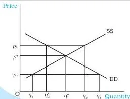
Take a price \( p_1 \) below \( p^* \). Demand \( q_1 \) exceeds supply \( q’_1 \), so excess demand of \( q_1 – q’_1 \) appears. Consumers who cannot buy the good are willing to pay more, so the price rises; as it rises, quantity demanded falls and quantity supplied rises. At a price \( p_2 \) above \( p^* \), supply \( q_2 \) exceeds demand \( q’_2 \) — excess supply of \( q_2 – q’_2 \).
Firms that cannot sell their desired output cut their prices; as the price falls, quantity demanded rises and quantity supplied falls. The adjustment stops only at \( p^* \), where the plans of both sides match (NCERT, pp. 72-73).
Equilibrium with a Fixed Number of Firms
Method. With a fixed number of firms, equilibrium is found by equating market demand and market supply (NCERT, p. 73):
\[ q^D(p^*) = q^S(p^*) \]
Solve for \( p^* \), then substitute it back into either equation to get \( q^* \). Graphically, this is the intersection of the market demand and supply curves.
Mind the price domains. The demand and supply functions in this chapter are defined only in specific price ranges (NCERT, p. 73). Demand is positive only up to a maximum price — above it, quantity demanded is zero. Supply is positive only from a minimum price upward — below it, firms supply nothing, since producing at such prices is not profitable.
In the textbook’s wheat example (Example 5.1), each function carries such a domain, and the equilibrium price must lie inside both. The same pattern reappears in the exercises, where supply is zero at any price below a stated minimum.
Once the market clears at \( p^* \), the gap between the two sides is itself a function of price:
- Excess demand: \( ED(p) = q^D – q^S \), positive for \( p \lt p^* \) and negative for \( p \gt p^* \).
- Excess supply: \( ES(p) = q^S – q^D \), positive for \( p \gt p^* \).
If the prevailing price is not \( p^* \), the market is out of equilibrium and the adjustment story of Figure 5.1 applies: excess demand pushes the price up, excess supply pulls it down, until \( p^* \) is reached.
The textbook’s worked example (p. 73) demonstrates the full method — equate demand to supply, solve for \( p^* \), substitute for \( q^* \), then confirm with the ED and ES functions that excess demand exists below \( p^* \) and excess supply above it.
How Shifts in Demand and Supply Move the Equilibrium
The demand and supply curves are drawn holding other factors constant: tastes and preferences, prices of related commodities, incomes of consumers, the size of the market, technology and input prices. A change in any of these shifts a curve and moves the equilibrium (NCERT, p. 76).
Demand Shift
Suppose the incomes of consumers rise. For a normal good such as clothes, consumers want more at every price, so the demand curve shifts rightward. An increase in the number of consumers has the same effect. This income change does not shift the supply curve — supply responds only to technology or cost-of-production factors (NCERT, p. 77).
A fall in income, or a fall in the number of consumers, shifts demand leftward.
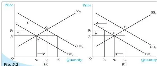
Figure 5.2 shows both directions with the supply curve fixed. In panel (a), the demand curve shifts right from \( DD_0 \) to \( DD_2 \). At the old price \( p_0 \) there is now excess demand, so price is bid up; the new equilibrium is at G with a higher price \( p_2 \) and a larger quantity \( q_2 \).
In panel (b), demand shifts left from \( DD_0 \) to \( DD_1 \); at \( p_0 \) there is excess supply, firms cut prices, and the new equilibrium F has a lower price \( p_1 \) and a smaller quantity \( q_1 \). The rule for any demand shift: price and quantity move in the same direction (NCERT, pp. 76-77).
Supply Shift
A rise in the price of an input raises each firm’s marginal cost, so at every price firms supply less: the supply curve shifts leftward. Demand is unaffected, because consumers’ demand does not depend on input prices directly (NCERT, p. 79). An increase in the number of firms, or a technological improvement, shifts supply rightward.
The textbook’s Figure 5.3 (not reproduced here) draws both cases. With a leftward shift from \( SS_0 \) to \( SS_2 \), the new equilibrium G sits at a higher price and a smaller quantity — excess demand at the old price pushes the price up.
With a rightward shift from \( SS_0 \) to \( SS_1 \), the new equilibrium F has a lower price and a larger quantity — excess supply at the old price pulls the price down. The rule for any supply shift: price and quantity move in opposite directions (NCERT, pp. 78-79).
Simultaneous Shifts
Both curves can shift at once, giving four possible combinations. Table 5.1 of the textbook summarises the effects (NCERT, pp. 79-80):
| Shift in demand | Shift in supply | Effect on quantity | Effect on price |
|---|---|---|---|
| Leftward | Leftward | Decreases | May increase, decrease or remain unchanged |
| Rightward | Rightward | Increases | May increase, decrease or remain unchanged |
| Leftward | Rightward | May increase, decrease or remain unchanged | Decreases |
| Rightward | Leftward | May increase, decrease or remain unchanged | Increases |
Memory device: when demand and supply shift in the same direction, the quantity effect is certain — both curves pull quantity the same way, so only the price effect is uncertain. When they shift in opposite directions, the price effect is certain — both curves pull price the same way, so only the quantity effect is uncertain.
If the two shifts are equal in size, one effect can disappear entirely. The textbook’s Figure 5.4 shows two special cases: in panel (a), both curves shift right, leaving price unchanged with a higher quantity; in panel (b), supply shifts right and demand shifts left, leaving quantity unchanged with a lower price (NCERT, p. 80).
Free Entry and Exit: Equilibrium at Minimum Average Cost
Now allow firms to enter or exit freely, and assume all firms are identical. The crucial implication: in equilibrium, no firm earns supernormal profit and no firm incurs a loss by staying in production.
- If price is above minimum average cost, firms earn supernormal profit. The opportunity attracts new firms; their entry shifts the supply curve rightward, the price falls, and the supernormal profit is wiped out.
- If price is below minimum average cost, firms earn less than normal profit. Some exit; the supply curve shifts leftward, the price rises, and profits recover to the normal level (NCERT, pp. 80-81).
Only at the price equal to minimum average cost does each firm earn normal profit — just enough to cover its explicit and opportunity costs — so no firm wants to enter or exit. Hence with free entry and exit, the equilibrium price is pinned down:
\[ p = \min AC \]
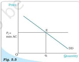
Figure 5.5 draws the outcome. The market demand curve DD cuts the horizontal line \( p_0 = \min AC \) at E. The equilibrium price is \( p_0 \), and the equilibrium quantity \( q_0 \) is simply the quantity demanded at that price. Every identical firm supplies the same output \( q_{0j} \) at \( p_0 \), so the equilibrium number of firms is (NCERT, p. 82):
\[ n_0 = \frac{q_0}{q_{0j}} \]
A demand shift changes quantity, not price. Suppose demand shifts right from \( DD_0 \) to \( DD_1 \) in the textbook’s Figure 5.6 (not reproduced here). At \( p_0 \) there is excess demand; price tends to rise, supernormal profit attracts new firms, and entry pushes the price back to \( p_0 \). The new equilibrium is at a larger quantity \( q_1 \), served by more firms.
A leftward shift works in reverse: excess supply at \( p_0 \) starts to pull the price down, losses drive some firms out, and the price returns to \( p_0 \) with a smaller quantity and fewer firms (NCERT, pp. 82-83).
So under free entry, a demand shift changes the equilibrium quantity and the number of firms in the same direction as the shift, but leaves price completely unchanged.
The same demand shift affects quantity more under free entry than under fixed firms, while price is not affected at all (NCERT, p. 83). The side-by-side comparison of the two regimes is in the Revision Summary at the end of this page.
Worked Examples: Solving Equilibrium Numericals Step by Step
Every linear demand-and-supply numerical uses the same skeleton: equate demand to supply at \( p^* \), solve for the price, substitute back for the quantity, then check the direction of change. The three examples below use original numbers — copy the steps and the shape of the working, not the values.
Example A: Equilibrium with a Fixed Number of Firms
Method: equate demand and supply, solve for \( p^* \), substitute back for \( q^* \).
Given: market demand \( q^D = 300 – 2p \) for \( 0 \leq p \leq 150 \); market supply \( q^S = 100 + 2p \) for \( p \geq 10 \).
Price is in rupees per kg and quantity in kg.
Step 1: Write the equilibrium condition \( q^D(p^*) = q^S(p^*) \).
\[ 300 – 2p^* = 100 + 2p^* \]
Step 2: Collect the \( p^* \) terms: \( 4p^* = 200 \), so \( p^* = 50 \).
The equilibrium price is Rs 50 per kg.
Step 3: Substitute \( p^* = 50 \) into the demand curve, and check with the supply curve.
\[ q^* = 300 – 2(50) = 200\ \text{kg} \quad \text{and} \quad q^* = 100 + 2(50) = 200\ \text{kg} \]
Step 4: Write the excess demand function.
\[ ED(p) = q^D – q^S = (300 – 2p) – (100 + 2p) = 200 – 4p \]
Step 5: Test the function on both sides of \( p^* \): at Rs 40 it must show excess demand, at Rs 60 excess supply.
\[ p = 40 \Rightarrow ED = 200 – 160 = 40\ \text{kg} \gt 0 \quad (\text{excess demand}) \]
\[ p = 60 \Rightarrow ED = 200 – 240 = -40\ \text{kg} \Rightarrow ES = 40\ \text{kg} \quad (\text{excess supply}) \]
Final answer: the market clears at \( p^* = \) Rs 50 per kg and \( q^* = 200 \) kg. Below Rs 50 excess demand is positive and above Rs 50 excess supply is positive, so equilibrium holds only at Rs 50.
Example B: Free Entry and Exit — Price, Quantity and Number of Firms
Method: with free entry, set price at minimum average cost, read the quantity from the market demand curve, then divide by the single firm’s supply.
Given: market demand \( q^D = 520 – 4p \); each identical firm’s supply is \( q_j = 10 + p \) for \( p \geq 30 \); minimum average cost is Rs 30.
Step 1: Free entry forces the price to minimum average cost: \( p_0 = 30 \).
Equilibrium price = Rs 30 per kg.
Step 2: Find the equilibrium quantity from the demand curve at \( p_0 \).
\[ q_0 = 520 – 4(30) = 520 – 120 = 400\ \text{kg} \]
Step 3: Find what one firm supplies at \( p_0 \).
\[ q_{0j} = 10 + 30 = 40\ \text{kg} \]
Step 4: Divide to get the equilibrium number of firms.
\[ n_0 = \frac{q_0}{q_{0j}} = \frac{400}{40} = 10 \]
Final answer: with free entry and exit, the equilibrium price is Rs 30 per kg, the equilibrium quantity is 400 kg, and 10 firms, each supplying 40 kg, serve the market.
Example C: A Supply Shift — Input Prices Rise
Method: replace the supply function with the new one, solve the equilibrium again, then compare with the old equilibrium.
Given: demand unchanged at \( q^D = 300 – 2p \).
Input prices rise, so the new market supply is \( q^S = 40 + 2p \) for \( p \geq 20 \).
Step 1: Equate the new supply with demand.
\[ 300 – 2p^* = 40 + 2p^* \]
Step 2: Solve: \( 4p^* = 260 \), so \( p^* = 65 \).
New equilibrium price = Rs 65 per kg.
Step 3: New equilibrium quantity:
\[ q^* = 300 – 2(65) = 170\ \text{kg} \]
Final answer: price rises from Rs 50 to Rs 65 per kg and quantity falls from 200 kg to 170 kg — price up, quantity down, exactly the rule for a leftward supply shift.
Wage Determination in the Labour Market
The labour market is the goods market in reverse: households supply labour and firms demand it. By “labour” the chapter means hours of work, not the number of labourers (NCERT, p. 74).
The hiring rule. The extra cost of hiring one more unit of labour is the wage \( w \). The extra benefit is the marginal revenue product of labour — the extra revenue earned from the output produced by that unit:
- \( MRP_L = MR \times MP_L \), marginal revenue times marginal product (NCERT, p. 75).
- For a perfectly competitive firm, \( MR = P \), so \( MRP_L = VMP_L = P \times MP_L \) — the value of marginal product of labour.
A profit-maximising firm employs labour up to the point where (NCERT, p. 75):
\[ w = MRP_L \]
Why labour demand slopes downward. By the law of diminishing marginal product, \( MP_L \) falls as employment rises. If the wage increases, the equality \( w = VMP_L \) can be restored only by employing less labour, where the marginal product is higher. So the market demand curve for labour — the sum of individual firms’ demands — slopes downward (NCERT, p. 75).
Why individual labour supply bends backward. A household chooses between income and leisure. A wage rise has two effects: it raises the opportunity cost of leisure, making leisure costlier (so the worker supplies more hours), and it raises purchasing power, making leisure more affordable (so the worker wants more of it).
At low wages the first effect dominates and labour supply rises with the wage; at high wages the second dominates and labour supply falls. The result is a backward bending individual supply curve (NCERT, p. 76).
Why the market supply curve still slopes upward. Aggregating across all households, many more individuals are attracted to supply labour at higher wages, even though some individuals work less. So the market labour supply curve is upward sloping (NCERT, p. 76).
With a downward-sloping labour demand and an upward-sloping labour supply, the equilibrium wage is determined at their intersection — the wage at which the labour households wish to supply equals the labour firms wish to hire (NCERT, p. 76). The textbook shows this in a labour-market diagram (not reproduced here).
Price Ceiling and Price Floor: Government Price Controls
Price controls are the chapter’s applications of demand-supply analysis. Both involve a government-imposed price different from the equilibrium price, and both create an imbalance that cannot clear the market (NCERT, p. 84).
Price Ceiling
A price ceiling is the government-imposed upper limit on the price of a good or service (NCERT, p. 84). It is generally imposed on necessary items — wheat, rice, kerosene, sugar — and is fixed below the market-determined price, so that a section of the population can afford them (NCERT, p. 84).
Figure 5.7 shows the wheat market. Left to itself, the market clears at the equilibrium \( (p^*, q^*) \). A ceiling \( p_c \) set below \( p^* \) changes the outcome: at \( p_c \), consumers demand \( q_c \) but firms are willing to supply only \( q’_c \), producing excess demand — a shortage of wheat.
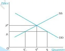
Misconception autopsy: does a price ceiling actually help consumers? The intention is to protect consumers, but the ceiling can end up hurting them in three ways (NCERT, pp. 84-85):
- A shortage appears: the quantity actually traded, \( q’_c \), is smaller than the free-market quantity \( q^* \).
- The scarce supply must be distributed — usually through rationing, with ration coupons that limit each consumer’s purchase through ration (fair price) shops.
- Consumers stand in long queues, and because the rationed quantity does not satisfy everyone, some are willing to pay more — a black market can arise.
Price Floor
A price floor is the government-imposed lower limit on the price that may be charged for a good or service (NCERT, p. 85). The two most well-known examples are agricultural price support programmes and minimum wage legislation; in both, the floor is fixed above the equilibrium price or wage (NCERT, p. 85).
Figure 5.8 shows the mechanics for a goods market. Equilibrium would be at \( (p^*, q^*) \). A floor \( p_j \) set above \( p^* \) makes firms want to supply \( q’_j \), while consumers demand only \( q_j \). The difference \( q_j q’_j \) is excess supply.
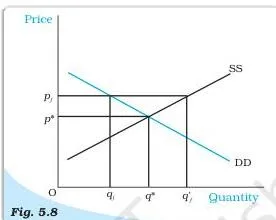
Under an agricultural support programme, the government must buy the surplus at the predetermined price to stop the price from falling again (NCERT, p. 85). Under minimum wage legislation, the wage is kept above the equilibrium wage so that it does not fall below a desired level.
| Price ceiling | Price floor | |
|---|---|---|
| Definition | Government-imposed upper limit on price | Government-imposed lower limit on price |
| Set relative to equilibrium | Below \( p^* \) | Above \( p^* \) |
| Resulting situation | Excess demand (shortage) | Excess supply (surplus) |
| How the imbalance is managed | Rationing through fair price shops | Government buys the surplus |
| Indian examples | Price controls on wheat, rice, kerosene, sugar (ration shops) | Minimum wage; agricultural support prices |
Key Terms and Definitions at a Glance
| Term | Meaning | Example |
|---|---|---|
| Equilibrium | A situation where the plans of all consumers and firms match and the market clears; market supply equals market demand (NCERT, p. 71). | The wheat market at the price where farmers’ supply equals consumers’ demand. |
| Equilibrium price | The price at which market demand equals market supply (NCERT, p. 71). | Rs 50 per kg in Example A. |
| Equilibrium quantity | The quantity bought and sold at the equilibrium price (NCERT, p. 71). | 200 kg in Example A. |
| Excess demand | Market demand greater than market supply at a price (NCERT, p. 72). | Consumers wanting more wheat than is supplied at a low price. |
| Excess supply | Market supply greater than market demand at a price (NCERT, p. 72). | Firms unable to sell all their wheat at a high price. |
| Marginal revenue product of labour \( (MRP_L) \) | The extra benefit of one more unit of labour: \( MR \times MP_L \) (NCERT, p. 75). | If \( MP_L = 4 \) units and \( MR = \) Rs 10, then \( MRP_L = \) Rs 40. |
| Value of marginal product of labour \( (VMP_L) \) | Product price times the marginal product of labour: \( P \times MP_L \) (NCERT, p. 75). | If \( P = \) Rs 10 and \( MP_L = 4 \), then \( VMP_L = \) Rs 40; equals \( MRP_L \) under perfect competition. |
| Backward bending labour supply curve | The individual supplies more labour as the wage rises only up to a point; beyond it, labour supply falls (NCERT, p. 76). | A worker takes on extra hours as overtime pay rises, then chooses more leisure at very high pay. |
| Normal profit | Profit just enough to cover explicit costs and opportunity costs (NCERT, p. 89). | A shopkeeper’s earnings that just match the salary she could earn elsewhere. |
| Supernormal profit | Profit over and above normal profit (NCERT, p. 90). | Earnings that exceed the opportunity costs of running a business. |
| Minimum average cost | The lowest point of the average cost curve; with free entry and exit the price equals it (NCERT, p. 81). | Rs 30 in Example B. |
| Price ceiling | Government-imposed upper limit on the price of a good or service (NCERT, p. 84). | Cap on the wheat price below the market equilibrium. |
| Price floor | Government-imposed lower limit on the price that may be charged (NCERT, p. 85). | Minimum wage set above the equilibrium wage. |
| Rationing | Distributing a limited quantity through coupons and fair price (ration) shops (NCERT, p. 84). | Wheat sold in limited amounts per coupon at a ration shop. |
Formulas: The Toolbox for Equilibrium Problems
All the quantitative relationships of the chapter in one place. Symbols: \( p \) = price (Rs per unit), \( q \) = quantity (kg or units), \( w \) = wage rate (Rs per hour), \( P \) = product price (Rs per unit).
| Relationship | Formula | What it means / when to use |
|---|---|---|
| Equilibrium condition | \( q^D(p^*) = q^S(p^*) \) | Solve this for the equilibrium price when the number of firms is fixed. |
| Excess demand | \( ED(p) = q^D – q^S \) | Positive below \( p^* \); tells which side of equilibrium the market is on. |
| Excess supply | \( ES(p) = q^S – q^D \) | Positive above \( p^* \). |
| Free-entry equilibrium price | \( p = \min AC \) | Under free entry, price settles at each identical firm’s minimum average cost. |
| Equilibrium number of firms | \( n_0 = \frac{q_0}{q_{0j}} \) | Total market quantity divided by one firm’s quantity, both taken at \( p_0 \). |
| Hiring rule | \( w = MRP_L \) | Firms hire labour until the wage equals the marginal revenue product of the last unit. |
| Marginal revenue product | \( MRP_L = MR \times MP_L \) | Extra revenue from one more unit of labour. |
| Value of marginal product | \( VMP_L = P \times MP_L \) | Equals \( MRP_L \) only under perfect competition, where \( MR = P \). |
Every numerical answer must carry units — a price without “Rs per kg” or a quantity without “kg” is incomplete.
Common Mistakes Students Make in This Chapter
Check your working against these six recurring errors.
| Students write… | Correct rule | How to check your answer |
|---|---|---|
| “Demand equals supply” as if it held at every price. | Demand equals supply at exactly one price — \( p^* \), where the curves intersect. At every other price there is excess demand or excess supply (NCERT, p. 72). | Plug \( p^* \) into \( q^D \) and \( q^S \) separately — the two values must match. |
| Calling a movement along a curve a “shift”. | A change in the good’s own price moves the point along the same curve. Income, number of consumers and tastes shift demand; input prices, technology and number of firms shift supply (NCERT, pp. 76-79). | Ask what changed: the price of the good itself (movement) or a non-price factor (shift)? |
| Ignoring the price ranges where supply is zero. | Check the domain before solving: demand is zero above a maximum price, supply is zero below a minimum price (NCERT, p. 73). | Confirm your \( p^* \) lies inside both domains. |
| Swapping the effects of price ceiling and price floor. | Ceiling below equilibrium \( \rightarrow \) excess demand; floor above equilibrium \( \rightarrow \) excess supply (NCERT, pp. 84-85). | Compare the control price with \( p^* \) first, then state the excess. |
| Assuming a price ceiling purely helps consumers. | It can also create a shortage, long queues and black markets; the quantity actually traded can fall below \( q^* \) (NCERT, pp. 84-85). | Compare the quantity supplied at the ceiling with the equilibrium quantity. |
| Confusing \( MRP_L \) with \( VMP_L \). | They are equal only under perfect competition, because \( MR = P \); in general \( MRP_L = MR \times MP_L \) while \( VMP_L = P \times MP_L \) (NCERT, p. 75). | Check whether the firm is a price-taker in the goods market before equating them. |
Exam Notes: How to Write Full Answers to This Chapter’s Exercises
The exercises of this chapter (NCERT, pp. 86-87) fall into six types. Each has a repeatable structure:
| Question type | Exercises | What a complete answer includes |
|---|---|---|
| Definition | 1, 2, 3 | The definition in your own words plus the condition: market demand equals market supply for equilibrium; one side exceeding the other for excess demand or excess supply. |
| Adjustment | 4 | Three steps: compare demand and supply at the given price, name the excess (demand or supply), then state the price movement back toward equilibrium. |
| Diagram | 5, 11, 15, 19 | Draw the demand and supply curves, label the initial and new equilibrium points, and state the direction of change in price and quantity. |
| Comparison | 14, 16, 21 | State the rule for each regime, then compare, using fixed-number-of-firms versus free-entry-and-exit language. |
| Numerical | 22, 23, 24 | The five-step method given below. |
| Application | 10, 11, 13, 20, 25 | Identify the relationship (substitute, complement or input), name the curve that shifts and its direction, then state the new equilibrium. |
Five-step method for numerical questions (exercises 22, 23, 24):
- Write the equilibrium condition \( q^D(p^*) = q^S(p^*) \).
- Substitute the given demand and supply functions.
- Solve for the equilibrium price \( p^* \).
- Substitute \( p^* \) back into either function to get \( q^* \).
- Interpret the result with units, and check the direction of any change against the shift rules.
For application questions, walk through the chain: identify the relationship between the goods or factors involved, name the curve that shifts and its direction, then state the new equilibrium. For definition and adjustment questions, keep the answer short but complete — every term you introduce needs its condition stated, not just a label.
Revision Summary in One Page
Along with the rest of our CBSE notes library, this page condenses the chapter’s own summary points (NCERT, pp. 85-86) into three quick tables.
Table 1 — What happens to price and quantity for each shift case (fixed number of firms):
| Shift case | Equilibrium price | Equilibrium quantity |
|---|---|---|
| Demand shifts right | Increases | Increases |
| Demand shifts left | Decreases | Decreases |
| Supply shifts right | Decreases | Increases |
| Supply shifts left | Increases | Decreases |
| Both shift right | May increase, decrease or remain unchanged | Increases |
| Both shift left | May increase, decrease or remain unchanged | Decreases |
| Demand right, supply left | Increases | May increase, decrease or remain unchanged |
| Demand left, supply right | Decreases | May increase, decrease or remain unchanged |
Table 2 — Fixed number of firms versus free entry and exit:
| Fixed number of firms | Free entry and exit | |
|---|---|---|
| Equilibrium condition | Market demand equals market supply (curves intersect) | Price equals minimum average cost: \( p = \min AC \) |
| Effect of a demand shift on price | Price changes in the same direction as the shift | Price remains unchanged |
| Effect of a demand shift on quantity | Quantity changes in the same direction as the shift | Quantity changes by more than under fixed firms |
| Effect on the number of firms | Number of firms is fixed | Number of firms changes in the same direction as demand |
Table 3 — Price ceiling versus price floor:
| Price ceiling | Price floor | |
|---|---|---|
| Definition | Upper limit on price | Lower limit on price |
| Position relative to equilibrium | Below \( p^* \) | Above \( p^* \) |
| Resulting situation | Excess demand (shortage) | Excess supply (surplus) |
| Examples | Price controls on essentials such as wheat and rice (ration shops) | Minimum wage; agricultural support prices |
Key results at a glance:
- In a perfectly competitive market, equilibrium occurs where market demand equals market supply; the invisible hand removes any excess demand or supply by changing price.
- With a fixed number of firms, a demand shift moves price and quantity in the same direction, while a supply shift moves them in opposite directions.
- When both curves shift in the same direction, the quantity effect is certain; when they shift in opposite directions, the price effect is certain.
- Each firm employs labour up to the point where the marginal revenue product of labour equals the wage rate.
- With free entry and exit of identical firms, the equilibrium price is \( p = \min AC \); a demand shift changes quantity and the number of firms but not price, and the quantity effect is stronger than with fixed firms.
- A price ceiling below the equilibrium price leads to excess demand; a price floor above the equilibrium price leads to excess supply (NCERT, pp. 85-86).
Frequently Asked Questions About Market Equilibrium
What is the difference between excess demand and excess supply?
Excess demand exists when market demand exceeds market supply at a given price; excess supply exists when market supply exceeds market demand at that price. At the equilibrium price both are zero — which is why equilibrium can be defined as a zero excess demand and zero excess supply situation (NCERT, p. 72).
Why is the equilibrium price equal to minimum average cost when firms can enter and exit freely?
Because any other price cannot persist. Above \( \min AC \), supernormal profit attracts new firms, shifting supply rightward and pulling the price down; below \( \min AC \), losses push firms to exit, shifting supply leftward and raising the price. Only at \( p = \min AC \) do all firms earn normal profit, with no incentive to enter or exit (NCERT, pp. 80-81).
What happens to equilibrium price and quantity when both demand and supply curves shift rightward?
The equilibrium quantity increases without ambiguity, but the price may increase, decrease or remain unchanged depending on the magnitudes of the two shifts (NCERT, Table 5.1, p. 80). If both curves shift right by the same amount, price stays unchanged while quantity rises.
Why does a price ceiling fixed below the equilibrium price create a shortage?
At the ceiling price, quantity demanded \( q_c \) exceeds quantity supplied \( q’_c \), so excess demand — a shortage — appears. Because the price is legally prevented from rising, the market cannot clear itself and the shortage persists (NCERT, p. 84).
How is the wage rate determined in a perfectly competitive labour market?
At the intersection of the market labour demand and supply curves. Firms’ demand for labour is determined by the hiring rule \( w = MRP_L \), and the wage settles where the hours households wish to supply equal the hours firms wish to hire (NCERT, pp. 74-76).
Why is the individual labour supply curve backward bending while the market supply curve is upward sloping?
The individual curve bends backward because at high wages the income effect — more purchasing power leads to more leisure — dominates the opportunity-cost effect, so the person works less. The market curve stays upward sloping because higher wages attract many more individuals into the labour force, which outweighs the reduced hours of some individuals (NCERT, p. 76).
Reference: NCERT Class 12 Economics textbook, chapter Market Equilibrium.
Explore Class 12 Economics Notes
- Class 12 Economics Notes
- Class 12 CBSE Notes
- CBSE Notes for Classes 1 to 12
- Previous: The Theory of the Firm under Perfect Competition
Class 12 Economics on LearnCBSE:
Related chapters:
- A Simple Economy notes
- Theory of Consumer Behaviour notes
- Production and Costs notes
Official source: download the NCERT textbook free from ncert.nic.in.