
When the price of final goods and the interest rate are both fixed, what decides how much a country produces and employs? That is the question this chapter answers. It builds the Keynesian theory of income determination: consumption and investment plans create aggregate demand, and output settles where planned demand equals planned output — not at any guaranteed level of employment.
These determination of income and employment class 12 notes compress the chapter for revision: ex ante and ex post values, the consumption function and the four propensities, the 45-degree diagram, the multiplier, the paradox of thrift, and the two demand gaps.
You get a definitions table, a formula sheet with every symbol explained, three worked examples with original numbers, a common-mistakes table, and answer structure for all six textbook exercises. These notes follow the 2026-27 session and the rationalised NCERT book.
The full NCERT Class 12 Introductory Macroeconomics textbook can be downloaded from the official NCERT textbook portal. This page is part of our Class 12 economics notes; wherever the model draws on tools you met earlier, those links are flagged so you can revise both together.
Reference: NCERT Class 12 Economics textbook, chapter Determination of Income and Employment.
The One Question This Chapter Answers
Macroeconomics cannot track every variable at once, so models isolate one target variable and hold the rest fixed. This is the ceteris paribus assumption — literally “other things remaining equal”. To find what determines national income, this chapter holds two things constant:
- Price of final goods is fixed. There are unused machines, buildings and labour, so extra output can be produced without pushing up marginal cost (NCERT, p. 57).
- Rate of interest is constant. What actually moves the interest rate is the money market, studied separately in our money and banking notes.
The model is the theory of John Maynard Keynes. The textbook works in two stages: first it solves for equilibrium with the price level fixed, then it allows the price level to vary (NCERT, p. 57). The whole chapter is one logical chain:
- Aggregate demand = planned consumption + planned investment.
- Equilibrium holds where planned demand equals planned output.
- Any autonomous change is multiplied, so income moves more than the initial spending change.
- Equilibrium can settle below or above full employment — creating deficient or excess demand.
Two simplifications keep the model clean. No indirect taxes or subsidies means GDP equals National Income, so the chapter uses one symbol, \(Y\), for both (NCERT, p. 57). And the government sector is introduced briefly — tax \(T\) and spending \(G\) as autonomous fiscal variables — only to be set aside; the fiscal variables return properly in the government budget chapter.
Exports and imports are also absent here; they enter the model in open economy macroeconomics.
Ex Ante and Ex Post: Planned Values Drive the Model
The whole chapter turns on one distinction. Ex ante values are planned values — what households plan to consume, what producers plan to invest, what output they plan to supply. Ex post values are actual, realised values, the ones national income accounting measures (NCERT, p. 54).
Try this inventory example. A producer plans to add Rs 200 worth of goods to stock by year-end. An unexpected sales surge forces her to sell Rs 150 from the stock she already holds. Her planned investment was Rs 200, but the net addition to inventory at year-end is only \(200 – 150 = 50\) rupees. So planned investment is Rs 200, while actual investment is Rs 50.
The gap appears because unplanned inventory investment occurred: sales exceeded the plan, so inventories were drawn down. Inventory investment can be positive (stock rising) or negative (stock being depleted), and it arises from two causes — deliberate stocking decisions (planned inventory investment) and sales that diverge from the plan (unplanned inventory investment) (NCERT, pp. 56-57).
Income determination uses ex ante values. In equilibrium, planned output equals planned demand. Outside equilibrium, actual output always equals actual demand — the difference shows up as unintended inventory accumulation. That is why the model’s equilibrium condition talks about plans, not measurements.
The Consumption Function and the Four Propensities
Household income is the main determinant of consumption demand, and the chapter assumes the simplest possible relation: consumption changes at a constant rate as income changes (NCERT, p. 54). The consumption function is \[ C = \bar{C} + cY \]
- Autonomous consumption \( \bar{C} \) — consumption that continues even at zero income, driven by subsistence needs. It is a constant.
- Induced consumption \( cY \) — the part that depends on income. For every Re 1 rise in income, induced consumption rises by \( c \), the marginal propensity to consume.
Since income is either consumed or saved, \( S = Y – C \). From this come the four propensities (NCERT, p. 55):
- MPC \( c = \frac{\Delta C}{\Delta Y} \) — the rate of change of consumption as income changes. Because consumption can never change by more than income, \( 0 \leq c \leq 1 \).
- MPS \( s = \frac{\Delta S}{\Delta Y} = 1 – c \) — the rate of change of savings as income changes; hence \( c + s = 1 \).
- APC \( = \frac{C}{Y} \) — consumption per unit of income.
- APS \( = \frac{S}{Y} \) — savings per unit of income.
Because \( C + S = Y \), dividing by \(Y\) gives \( APC + APS = 1 \). Quick check: with \( \bar{C} = 60 \) and \( c = 0.75 \), an income rise of 40 raises consumption by 30 and savings by 10 — MPC 0.75, MPS 0.25, and \( 0.75 + 0.25 = 1 \).
Investment in This Model: The Autonomous Investment Line
Investment means additions to physical capital — machines, buildings, roads — plus changes in a producer’s inventory of finished goods. Investment goods are final goods, not intermediate goods: a machine is not used up in producing other goods but yields its services over several years (NCERT, p. 56).
Real-world investment depends on factors like the availability of credit and the market rate of interest. The chapter simplifies: firms plan the same investment every year, so ex ante investment is a positive constant (NCERT, p. 56):
\[ I = \bar{I} \]
This is autonomous investment — given from outside the model and independent of income. Its graph is shown in Fig. 4.3: a horizontal line at height \( \bar{I} \) above the income axis, meaning planned investment is the same at every income level.
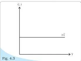
The chapter names two real-world drivers of investment that would move \( \bar{I} \) — easy availability of credit encourages investment, and higher interest rates discourage it — but treats them as outside this model.
Equilibrium Income: The 45-Degree Diagram and the Algebra
In a two-sector economy — households and firms, no government — planned aggregate demand is the sum of planned consumption and planned investment:
\[ AD = \bar{C} + \bar{I} + cY = \bar{A} + cY \]
where \( \bar{A} = \bar{C} + \bar{I} \) is total autonomous expenditure. The chapter notes that \( \bar{C} \), representing subsistence consumption, stays stable over time, while \( \bar{I} \) undergoes periodic fluctuations (NCERT, p. 56).
Graphical method: from the intercept form to the AD line
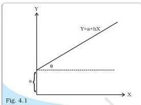
The graph starts from the intercept form of a linear equation, \( Y = a + bX \): the constant \( a \) is the intercept (the value of Y when X is zero) and \( b \) is the slope. Fig. 4.1 shows exactly this — a straight line cutting the vertical axis at \( a \) and rising with slope \( b \).
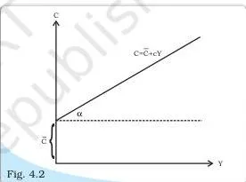
The consumption function is the same picture renamed. In Fig. 4.2 the consumption line cuts the vertical axis at \( \bar{C} \) — autonomous consumption — and its slope is the MPC, \( c = \tan \alpha \).
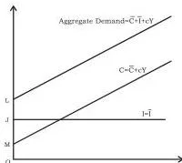
Aggregate demand adds investment to consumption. Fig. 4.4 shows the vertical addition of the two functions: the vertical-axis distances give autonomous consumption \( \bar{C} \), autonomous investment \( \bar{I} \), and their sum \( \bar{C} + \bar{I} \). The AD line is parallel to the consumption line — the same slope \( c \) — and it represents ex ante demand (NCERT, p. 59).
The 45-degree line is the supply side
The supply side is drawn as a 45-degree line. Every point on a line at \( 45^\circ \) to the axes has equal horizontal and vertical coordinates, so it maps each level of planned output to an equal quantity on the demand axis.
At a GDP of Rs 1,000 at point A, the quantity supplied is found at the point B directly above A on the 45-degree line — Rs 1,000 worth of goods (NCERT, p. 59). Because the price is fixed and unused resources exist, supply is assumed perfectly elastic; output moves up or down freely.
The intersection of the AD line with the 45-degree line is equilibrium: there, ex ante aggregate demand equals ex ante aggregate supply. (Figs 4.5 and 4.6 in the textbook draw the 45-degree supply line and the equilibrium intersection; the logic is exactly as described here.)
Algebraic method: solving for equilibrium Y
Set ex ante supply equal to ex ante demand (NCERT, p. 60):
\[ Y = \bar{C} + \bar{I} + cY \]
\[ Y(1 – c) = \bar{C} + \bar{I} \]
\[ Y = \frac{\bar{C} + \bar{I}}{1 – c} = \frac{\bar{A}}{1 – c} \quad (4.4) \]
Equilibrium condition, not an accounting identity
A caution that trips many students: this \( Y = AD \) equation is NOT the accounting identity of Chapter 2. The identity always holds for actual (ex post) values — that is the identity you met in national income accounting. Equation (4.3) here holds only for planned (ex ante) values, and only in equilibrium.
If planned demand falls short of planned output, stocks pile up as unintended inventory accumulation; actual output still equals actual demand because the unsold output is counted in ex post inventory investment (NCERT, pp. 56-57).
The model also uses the idea of a parametric shift: a change in a parameter of the model. Raise a parameter like \( \bar{A} \) (the intercept) and the line shifts up in parallel; reduce \( c \) (the slope) and the line swings down. The next sections use both movements.
Revise by redrawing
To revise from these diagrams, redraw each one and label: Fig. 4.1 — intercept \(a\) and slope \(b\); Fig. 4.2 — intercept \( \bar{C} \) and slope \( c \); Fig. 4.3 — constant height \( \bar{I} \); Fig. 4.4 — the vertical gap of \( \bar{I} \) between the consumption line and the AD line, with equal slopes; Fig. 4.7 — the excess demand gap and the income increase (below).
Autonomous Change and the Multiplier Mechanism
Effect of an autonomous change in spending
Because equilibrium income depends on aggregate demand, a rise in autonomous investment shifts the whole AD line upward in parallel. At the old equilibrium there is now excess demand: Fig. 4.7 labels it \( E_1F \) — the gap between the new AD line and the old output level. The economy then moves up the 45-degree line to the new intersection \( E_2 \).
Two distances in Fig. 4.7 carry the meaning (NCERT, p. 61):
- \( E_1F \) is the initial excess demand, equal to the rise in autonomous expenditure \( \Delta \bar{I} \);
- \( E_1G = E_2G \) is the total increase in output and demand — and it is larger than \( \Delta \bar{I} \).
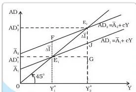
So a small autonomous change produces a bigger change in income. That is the multiplier, explained round by round below.
The round-by-round mechanism
Extra output pays extra factor incomes — wages, interest, rent, profit — and part of that income is spent again as consumption, which raises demand, which raises output, which raises income again. One autonomous change thus ripples through the circular flow. Example: investment rises by 20 and mpc = 0.6.
| Round | Extra demand created | Extra output / income |
|---|---|---|
| Round 1 | 20 (autonomous investment) | 20 |
| Round 2 | \( 0.6 \times 20 = 12 \) | 12 |
| Round 3 | \( 0.6 \times 12 = 7.2 \) | 7.2 |
| Round 4 | \( 0.6 \times 7.2 = 4.32 \) | 4.32 |
| … | each round, 0.6 of the previous | total \( \frac{20}{1 – 0.6} = 50 \) |
Why does the chain converge? In each round, a fraction of extra income is saved and not re-spent; saving is the leakage that shrinks the successive rounds.
The multiplier formula
The ratio of the total increase in equilibrium output to the initial autonomous change is the investment multiplier, also called the autonomous expenditure multiplier (NCERT, p. 62):
\[ \frac{\Delta Y}{\Delta \bar{A}} = \frac{1}{1 – c} = \frac{1}{s} \quad (4.5) \]
where \( c \) = MPC and \( s \) = MPS. The multiplier is the reciprocal of the MPS because \( s \) is the fraction of each income increment that leaks out of the spending chain every round. The larger the MPC, the larger the multiplier — more of each round’s income returns to the market as demand.
Note that \( \Delta \bar{I} = \Delta \bar{A} \), since investment is a component of autonomous expenditure.
Paradox of Thrift: More Saving, Same Savings
The paradox of thrift: when all people in the economy try to save a larger proportion of their income, total savings do not rise — they stay the same or fall (NCERT, p. 63). The mechanism runs like this:
- People become more thrifty, so MPS rises and MPC falls. At the old income, consumption demand drops — like an autonomous fall in demand.
- Demand falls short of output, stocks pile up, and producers cut output.
- Lower output means lower factor payments and lower income, which cuts consumption again — and the chain repeats.
Work it with fresh numbers. Start with \( \bar{C} = 50 \), \( \bar{I} = 30 \) (so \( \bar{A} = 80 \)), and \( c = 0.8 \):
\[ Y = \frac{80}{1 – 0.8} = 400, \qquad S = Y – C = 400 – (50 + 0.8 \times 400) = 30 \]
Now mpc falls to 0.6 (mps rises from 0.2 to 0.4). At the old income of 400, the mpc fall cuts consumption demand by \( (0.8 – 0.6) \times 400 = 80 \). This initial demand fall triggers the convergent series of further falls — each later income cut reduces consumption by 0.6 of the previous one:
\[ \Delta Y = 80 + (0.6)80 + (0.6)^2 80 + \dots = \frac{80}{1 – 0.6} = 200 \]
\[ Y = 400 – 200 = 200, \qquad S = 200 – (50 + 0.6 \times 200) = 30 \]
Income fell from 400 to 200, yet total savings stayed at 30. The higher saving rate is applied to a much lower income, so the absolute level of saving does not rise.
Note the shift-versus-swing contrast. When \( \bar{A} \) changes, the AD line shifts up or down in parallel. When \( c \) changes, the line swings about its intercept; Fig. 4.8 in the textbook (not reproduced here) draws this downward swing of the AD line.
A rise in MPS reduces the slope of AD, and the swinging line meets the 45-degree line at a lower income.
Full Employment, Deficient Demand and Excess Demand
Equilibrium is not the same as full employment. Equilibrium only means income has no tendency to change; it can coexist with unemployment. The full-employment level of income is the level at which all factors of production are fully employed (NCERT, p. 64).
- Deficient demand — equilibrium income is below the full-employment level because demand is too low to employ all factors. Its long-run effect is falling prices.
- Excess demand — equilibrium income is above the full-employment level because demand exceeds what can be produced at full employment. Its long-run effect is rising prices.
Memory device: deficient demand pairs with deflation — both start with “de” — while excess demand pairs with rising prices: extra demand pushes prices up.
Key Definitions at a Glance
The chapter’s full terminology in two tables. The first packs every concept; the second isolates the four propensities for direct comparison.
| Term | Meaning | Example or remark |
|---|---|---|
| Ex ante | Planned values of consumption, investment or output | A producer’s planned inventory addition |
| Ex post | Actual, realised values as recorded | The inventory addition that actually happened |
| Autonomous consumption \( \bar{C} \) | Consumption that takes place even at zero income | Subsistence consumption; a constant |
| Induced consumption \( cY \) | The part of consumption that varies with income | Rises by \( c \) for each Re 1 of income |
| MPC \( c \) | Change in consumption per unit change in income, \( \frac{\Delta C}{\Delta Y} \) | \( 0 \leq c \leq 1 \) |
| MPS \( s \) | Change in savings per unit change in income, \( \frac{\Delta S}{\Delta Y} \) | \( s = 1 – c \), so \( c + s = 1 \) |
| APC | Consumption per unit of income, \( \frac{C}{Y} \) | Average ratio; unitless |
| APS | Savings per unit of income, \( \frac{S}{Y} \) | \( APS = 1 – APC \) |
| Autonomous investment \( \bar{I} \) | Planned investment treated as a positive constant | Independent of income |
| Unintended inventory accumulation | Stock that piles up when planned demand falls short of planned output | Restores the ex post identity |
| Parametric shift | A change in a parameter of the model | Intercept change → parallel shift; slope change → swing |
| Effective demand | Principle that, with fixed price and elastic supply, output is determined by aggregate demand | Output is demand-determined |
| Autonomous expenditure multiplier | \( \frac{\Delta Y}{\Delta \bar{A}} = \frac{1}{1 – c} \) | Also equals \( \frac{1}{s} \) |
| Paradox of thrift | A rise in the economy’s MPS leaves total savings unchanged or lower | Income falls faster than the saving rate rises |
| Deficient demand | Equilibrium income below full-employment income | Long-run effect: falling prices |
| Excess demand | Equilibrium income above full-employment income | Long-run effect: rising prices |
| Full employment | Income level at which all factors of production are fully employed | Equilibrium need not equal it |
The four propensities compared
| Propensity | Formula | What it measures | Property |
|---|---|---|---|
| MPC | \( c = \frac{\Delta C}{\Delta Y} \) | Change in consumption per unit change in income | \( 0 \leq c \leq 1 \) |
| MPS | \( s = \frac{\Delta S}{\Delta Y} \) | Change in savings per unit change in income | \( c + s = 1 \) |
| APC | \( \frac{C}{Y} \) | Consumption per unit of income | \( APC + APS = 1 \) |
| APS | \( \frac{S}{Y} \) | Savings per unit of income | \( APS = 1 – APC \) |
MPC and MPS are marginal — about changes; APC and APS are average — about levels. Each pair sums to 1 because every extra rupee of income is either consumed or saved, and every rupee of income is either one or the other.
Formula Sheet: Every Equation and What It Means
All the equations of the chapter in one table, with each symbol and unit spelled out.
| Formula | Symbol meanings | Key property / unit |
|---|---|---|
| \( C = \bar{C} + cY \) | \( \bar{C} \): autonomous consumption; \( c \): MPC; \( Y \): income | Consumption in Rs (crores); \( 0 \leq c \leq 1 \) |
| \( S = Y – C \) | \( S \): savings, the part of income not consumed | Savings in Rs (crores) |
| \( c = \frac{\Delta C}{\Delta Y} \) | Rate of change of consumption with respect to income | Unitless ratio |
| \( s = \frac{\Delta S}{\Delta Y} = 1 – c \) | Rate of change of savings with respect to income | Unitless; \( c + s = 1 \) |
| \( APC = \frac{C}{Y} \) | Consumption per unit of income | Unitless average |
| \( APS = \frac{S}{Y} \) | Savings per unit of income | Unitless; \( APC + APS = 1 \) |
| \( I = \bar{I} \) | \( \bar{I} \): autonomous (given) investment | Positive constant; Rs (crores) |
| \( AD = \bar{C} + \bar{I} + cY = \bar{A} + cY \) | \( \bar{A} = \bar{C} + \bar{I} \): total autonomous expenditure | Planned (ex ante) demand, two-sector economy |
| \( Y = \frac{\bar{C} + \bar{I}}{1 – c} = \frac{\bar{A}}{1 – c} \) | \( Y \): equilibrium income | Holds only when ex ante demand equals supply (4.4) |
| \( \frac{\Delta Y}{\Delta \bar{A}} = \frac{1}{1 – c} = \frac{1}{s} \) | Investment / autonomous expenditure multiplier | Unitless; larger when \( c \) is larger (4.5) |
| \( Y = \bar{C} + \bar{I} + G + c(Y – T) \) | \( G \): government spending; \( T \): taxes; \( Y_d = Y – T \): disposable income | With-government setup; then the chapter sets \( G = T = 0 \) |
Units to remember: income, consumption, investment and savings are rupee amounts (typically crores in numerical problems). MPC, MPS, APC, APS and the multiplier are unitless ratios.
Worked Examples: Three Problems Solved Step by Step
Work each problem with pen and paper before reading the steps. The numbers here are original to these notes.
Example 1: Planned vs actual inventory investment
Method: separate planned from actual by tracking the inventory change.
Step 1: A producer plans to add Rs 200 worth of goods to stock by year-end.
Planned (ex ante) investment = Rs 200.
- Step 1: An unexpected sales surge forces her to sell Rs 150 from existing stock — an unplanned inventory drawdown of Rs 150.
- Step 2: Net inventory investment = \( 200 – 150 = 50 \) rupees.
This is the actual (ex post) investment.
Final answer: planned investment is Rs 200 and actual investment is Rs 50. The Rs 150 difference is unplanned inventory investment (a depletion), which made ex post investment differ from the plan.
Example 2: Equilibrium income, then a multiplier effect
Method: use \( Y = \frac{\bar{A}}{1 – c} \) to find equilibrium, verify with \( S = I \), then apply the multiplier to the change in autonomous investment.
- Step 1: Given \( C = 60 + 0.75Y \) and \( \bar{I} = 40 \): here \( \bar{C} = 60 \), \( c = 0.75 \), so \( \bar{A} = 60 + 40 = 100 \) (Rs crore).
- Step 2: Equilibrium income:
\[ Y = \frac{\bar{A}}{1 – c} = \frac{100}{1 – 0.75} = \frac{100}{0.25} = 400 \]
Step 3: Verify \( S = I \) at equilibrium: \( C = 60 + 0.75(400) = 360 \), so \( S = 400 – 360 = 40 \), which equals planned \( \bar{I} = 40 \).
Equilibrium holds.
Step 4: Investment rises by \( \Delta \bar{I} = 15 \).
The multiplier is \[ \frac{1}{1 – c} = \frac{1}{1 – 0.75} = \frac{1}{0.25} = 4 \]
Step 5: \( \Delta Y = 4 \times 15 = 60 \), so the new equilibrium is \( 400 + 60 = 460 \) (Rs crore).
Check: at 460, \( C = 60 + 0.75(460) = 405 \), \( S = 55 = 40 + 15 \), the new total investment.
Round-by-round check of ΔY = 60:
| Round | Extra demand in the round | Extra output / income |
|---|---|---|
| Round 1 | 15 | 15 |
| Round 2 | \( 0.75 \times 15 = 11.25 \) | 11.25 |
| Round 3 | \( 0.75 \times 11.25 = 8.4375 \) | 8.4375 |
| … | each round, 0.75 of the previous | total \( \frac{15}{1 – 0.75} = 60 \) |
Final answer: equilibrium income rises from Rs 400 crore to Rs 460 crore — a gain of Rs 60 crore from a Rs 15 crore autonomous investment increase.
Example 3: Is the economy in equilibrium?
Method: compute planned aggregate demand at the given income and compare it with planned output; then find the equilibrium income for confirmation.
Step 1: Given autonomous expenditure \( \bar{A} = 120 \), MPS = 0.2, and income \( Y = 800 \) (Rs crore).
First find \( c = 1 – \text{MPS} = 1 – 0.2 = 0.8 \).
Step 2: Planned aggregate demand at \( Y = 800 \):
\[ AD = \bar{A} + cY = 120 + 0.8(800) = 120 + 640 = 760 \]
Step 3: Compare: planned AD (760) is less than planned output (800).
Output exceeds demand by 40, so the economy is not in equilibrium; Rs 40 crore of output piles up as unintended inventory accumulation.
Step 4: Confirm with the equilibrium formula:
\[ Y = \frac{\bar{A}}{1 – c} = \frac{120}{1 – 0.8} = 600 \]
Final answer: not in equilibrium. At \( Y = 800 \), aggregate demand is 760, giving excess supply of 40. The equilibrium income is 600, where \( AD = 120 + 0.8(600) = 600 \).
Common Mistakes and How to Fix Them
These are the errors this chapter reliably produces. Each row gives the mistake, the correct rule, and a quick way to check yourself.
| Mistake | Correct rule | How to check your answer |
|---|---|---|
| Writing APC where MPC is meant | APC is \( \frac{C}{Y} \), an average at a point; MPC is \( \frac{\Delta C}{\Delta Y} \), a rate of change | Ask: does the problem talk about a change in income, or a level? |
| Claiming MPC can exceed 1 | \( 0 \leq c \leq 1 \), because consumption can never change by more than income | Compute \( \frac{\Delta C}{\Delta Y} \); it cannot exceed 1 |
| Writing the multiplier as \( \frac{1}{c} \) | Multiplier is \( \frac{1}{1 – c} = \frac{1}{s} \) | Test \( c = 0.8 \): \( \frac{1}{0.8} = 1.25 \), but the true multiplier is 5 |
| Treating \( Y = AD \) as the Chapter 2 identity | It is an equilibrium condition on planned values; the identity always holds ex post | Ask “planned or actual?” — outside equilibrium the two differ through inventories |
| Confusing a slope change with an intercept change | Change in \( \bar{A} \) → parallel shift; change in \( c \) → the line swings | Identify which parameter moved before drawing |
| Concluding thrift always raises total savings | Paradox of thrift: the income fall offsets the higher saving rate | Recompute savings at the new, lower equilibrium income |
| Treating equilibrium as full employment | Equilibrium only means income will not change; it can sit below or above full employment | Compare equilibrium income with the full-employment level |
| Mixing up \( S \) and \( s \) | \( S \) is the rupee level of savings; \( s \) is MPS, a unitless ratio | Check units: \( S \) in rupees, \( s \) has no unit |
Answering the Textbook Exercises: What Each Question Wants
The six exercises at the end of the chapter (NCERT, p. 65) each check one idea. Below is the structure a complete answer should contain — work the numbers yourself.
- Exercise 1 (MPC and MPS): define MPC as the change in consumption per unit change in income, \( \frac{\Delta C}{\Delta Y} \); then state \( MPS = 1 – MPC \) and give the reason — every extra unit of income is either consumed or saved.
- Exercise 2 (ex ante vs ex post investment): define ex ante as planned and ex post as actual; illustrate with the inventory logic — planned stocking versus the actual stock change when sales diverge from the plan.
- Exercise 3 (parametric shift): define a parametric shift as a change in a parameter of the model; then state the two cases — slope decreases → the line swings down; intercept increases → the line shifts up in parallel.
- Exercise 4 (effective demand and the multiplier): state the effective demand principle — with fixed price and perfectly elastic supply, output is determined by aggregate demand; then derive the multiplier: set \( Y = \bar{A} + cY \), rearrange to \( Y = \frac{\bar{A}}{1 – c} \), so \( \frac{\Delta Y}{\Delta \bar{A}} = \frac{1}{1 – c} \).
- Exercise 5 (equilibrium check): write the AD equation, substitute the given autonomous expenditure, MPC (from \( c = 1 – \) MPS) and income; compare planned AD with \( Y \); conclude whether equilibrium holds, and give the reason in terms of unintended inventory accumulation.
- Exercise 6 (paradox of thrift): state the result; show the mechanism — higher MPS cuts consumption demand → excess supply → output and income fall → savings do not rise; close by noting that income is lower at the new equilibrium.
Revision Summary: The Chapter in One Page
The whole model in six steps:
- Planned (ex ante) values decide income — not ex post measurements.
- Build demand from \( C = \bar{C} + cY \) and \( I = \bar{I} \).
- Equilibrium is where planned output equals planned aggregate demand — the 45-degree crossing.
- Autonomous changes ripple through the multiplier \( \frac{1}{1 – c} \).
- Paradox of thrift: a higher MPS need not raise total savings.
- Equilibrium can settle below (deficient demand) or above (excess demand) full employment.
| Concept | One-line meaning | Formula / result |
|---|---|---|
| Autonomous consumption | Consumption that occurs even at zero income | \( \bar{C} \) in \( C = \bar{C} + cY \) |
| MPC | Extra consumption per extra rupee of income | \( c = \frac{\Delta C}{\Delta Y} \), \( 0 \leq c \leq 1 \) |
| Equilibrium income | Planned output equals planned demand | \( Y = \frac{\bar{A}}{1 – c} \) |
| Multiplier | Income change per unit autonomous change | \( \frac{1}{1 – c} = \frac{1}{s} \) |
| Paradox of thrift | More thrift, same savings | Income falls as MPS rises |
| Deficient demand | Equilibrium below full employment | Prices fall in the long run |
| Excess demand | Equilibrium above full employment | Prices rise in the long run |
For the full revision set, browse our Class 12 notes or the wider CBSE notes collection.
Frequently Asked Questions
Why is the aggregate supply curve drawn as a 45 degree line in this chapter?
Because every point on a 45-degree line has equal horizontal and vertical coordinates (NCERT, p. 59). Measure income along the horizontal axis; the point on the 45-degree line directly above any income level carries the same value on the vertical axis. So the line maps each planned output to an equal quantity of goods supplied at that GDP.
With the price fixed and unused resources available, supply is perfectly elastic — which is why the 45-degree line can serve as the aggregate supply curve.
Why is the investment multiplier equal to 1 divided by MPS?
Start from the equilibrium equation \( Y = \frac{\bar{A}}{1 – c} \). A change in autonomous spending \( \Delta \bar{A} \) changes income by \( \Delta Y = \frac{\Delta \bar{A}}{1 – c} \), so the multiplier is \( \frac{1}{1 – c} \). Since MPS \( s = 1 – c \), this is also \( \frac{1}{s} \).
The economic reason: each round, a fraction \( s \) of new income is saved and does not return to the spending stream, so the sum of all rounds is \( \frac{1}{s} \) times the initial injection.
What is the difference between deficient demand and excess demand?
Deficient demand is a situation where equilibrium income is below the full-employment level — demand is too low to employ all factors of production — and it leads to falling prices in the long run.
Excess demand is the opposite: equilibrium income is above the full-employment level because demand exceeds full-employment output, and it leads to rising prices in the long run (NCERT, p. 64). Both terms describe the gap between the actual equilibrium and the full-employment equilibrium, not an accounting shortfall.
How can people save more yet total savings stay the same in the paradox of thrift?
Because the attempt to save more lowers income. In the example from these notes: \( \bar{A} = 80 \), \( c = 0.8 \) gives \( Y = 400 \) and \( S = 30 \). When mpc falls to 0.6, consumption demand drops, output and income fall to 200, and savings are still 30. The higher saving rate is cancelled by the lower income at which it is applied.
The initial demand fall is \( (0.8 – 0.6) \times 400 = 80 \), and the convergent series \( \frac{80}{1 – 0.6} = 200 \) gives the total income fall (NCERT, p. 63).
What is effective demand in macroeconomics?
In this chapter, effective demand is the principle that aggregate output is determined solely by the level of aggregate demand (NCERT, p. 65). It holds under the chapter’s assumptions — a fixed price of final goods and perfectly elastic aggregate supply — so the demand the economy plans also sets the output.
The equilibrium output is therefore the level of demand that is “effective” in the market.
How do you check whether an economy is in equilibrium when you know autonomous expenditure, MPS and income?
Compute the MPC as \( c = 1 – \) MPS, then find planned aggregate demand \( AD = \bar{A} + cY \) at the given income. If AD equals Y, the economy is in equilibrium. If AD is less than Y, demand falls short and there is excess supply with unintended inventory accumulation; if AD exceeds Y, there is excess demand.
You can also compare the given Y with the equilibrium level \( \frac{\bar{A}}{1 – c} \); the economy is in equilibrium only when they match.
Reference: NCERT Class 12 Economics textbook, chapter Determination of Income and Employment.
Explore Class 12 Economics Notes
- Class 12 Economics Notes
- Class 12 CBSE Notes
- CBSE Notes for Classes 1 to 12
- Previous: Money and Banking
- Next: Open Economy Macroeconomics
Class 12 Economics on LearnCBSE:
Related chapters:
- National Income Accounting notes