
These genome engineering class 12 notes condense NCERT Class 12 Biotechnology Chapter 5 — titled “Genome Technology and Engineering” in the textbook — into one revision sitting. The chapter works as a single pipeline: know the genome, map it, sequence it, analyse it, engineer it, and finally engineer its proteins. Everything on this page follows the rationalised NCERT for the 2026-27 session.
Here is what you get, in teaching order: the genome’s definition and composition, genetic and physical mapping with their landmarks, the three generations of DNA sequencing and their variations, transposon and CRISPR-Cas9 engineering, the three branches of genomics, and the chapter’s four engineered proteins.
Each dense section ends in a comparison table, and three original worked examples show how the chapter’s rules are actually applied.
To revise fast, read each section together with its table, attempt the worked examples before reading the steps, then finish with the revision summary and the six-point self-check. This page is part of our Class 12 Biotechnology notes, which sit inside the wider Class 12 notes in the CBSE notes library.
Related biotechnology pages, such as our plant tissue culture notes, are linked from that hub. If you need the full chapter text, it is available on the official NCERT textbook portal. All page citations below refer to the NCERT Class XII Biotechnology textbook.
Chapter 5 at a Glance: The Genome Pipeline in Six Steps
The chapter’s six sections build on each other in exactly this order, and the chapter’s own summary on pages 136–137 confirms the pipeline below.
Pipeline: know the genome → map it → sequence it → analyse it → engineer it → engineer its proteins.
| Section | Title | Pages | Core idea |
|---|---|---|---|
| 5.1 | Mapping of the Genome: Genetic and Physical | 113–118 | Genetic maps built from recombination; physical maps built from DNA landmarks |
| 5.2 | High-throughput DNA sequencing | 118–124 | Three generations: chain termination, Illumina bridge PCR, nanopore |
| 5.3 | Other genome-related technology | 124–126 | WGS, targeted and clinical exome sequencing, ChIP-seq, RNA-seq, metagenomics |
| 5.4 | Genome Engineering | 126–129 | Transposon knock-out/knock-in; CRISPR-Cas9 editing |
| 5.5 | Structural, Functional and Comparative Genomics | 130–132 | Three branches that interpret genome sequences |
| 5.6 | Protein Engineering | 132–135 | Subtilisin, 6-His-tag, GFP, immunotoxin and humanised antibodies |
The Genome: The Material Chapter 5 Works With
A genome is the complete genetic information present in the cell of an organism (NCERT, p. 113). It is the material every technique in this chapter acts on: mapping orders it, sequencing reads it, and engineering edits it.
| Prokaryotes | Eukaryotes | |
|---|---|---|
| Where the DNA lives | Nucleoid region and plasmid (as in bacteria) | Chromosomes of the nucleus plus organelles — mitochondria and plastids such as chloroplasts |
| Example organisms | Bacteria | Protists and all multicellular organisms |
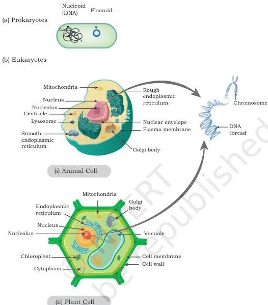
Figure 5.1 shows the two arrangements side by side. Panel (a) is a prokaryotic cell — its genome is the DNA of the nucleoid region plus the plasmid.
Panel (b) is a eukaryotic cell — its genome is the DNA of the nuclear chromosomes plus the DNA of organelles such as mitochondria and chloroplast; this layout covers protists and all multicellular organisms (NCERT, p. 114).
Why do biologists need to map and compare genomes at all?
The textbook’s motive (NCERT, p. 115) is practical: scientists want to understand conserved genes or DNA sequences and evolutionary relationships; they want to know whether DNA samples from two sources are similar or different and in what way; and when an interesting phenotype appears, they want its genetic basis — the genes and mutations behind it.
The chapter also assumes you know from Class XI how genetic information is encoded in DNA and how transcription and translation work (NCERT, p. 113); genome technology is essentially those processes handled at scale.
Genetic and Physical Mapping: Two Maps, Two Units
The distinction students miss first is a question of units. A genetic map measures relative distance by recombination frequency; a physical map identifies positions using actual DNA-based landmarks. One is built from what happens to phenotypes during crossing over; the other, from features detected directly in the DNA.
Genetic mapping rests on these points (NCERT, p. 115):
- Built from crossover analysis of loci responsible for a set of well-known phenotypes.
- The recombination frequency between two loci measures their relative genetic distance.
- Chances of two loci separating by recombination are directly proportional to the distance between them — so a smaller recombinant fraction means the loci are closer together.
- One map unit equals 1% of observed recombinants; the unit of genetic distance is the centimorgan (cM).
- Drawback: few loci have well-known phenotypes, so genetic maps stay sparsely populated, or coarsely grained, and cannot finely map a new phenotype onto the genome.
Physical mapping instead uses DNA-based map features — restriction enzyme sites (restriction mapping), Simple Sequence Length Polymorphism (SSLP) and Sequence Tagged Sites (STS) — which together give a high-resolution physical map (NCERT, p. 116).
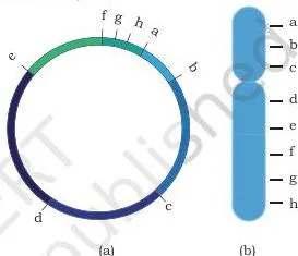
Figure 5.2 shows the two shapes a genome map can take: (a) a circular map for a prokaryotic or organelle genome, and (b) the linear arrangement of a eukaryotic genome, where the labels a–h represent genetic loci or physical sites such as SSLP and STS placed according to their mapped distances.
Misconception autopsy — why genetic maps stay coarse and physical maps go fine: a genetic map can only use loci whose phenotypes are already well characterised, and there are few of them, so its landmarks sit far apart. A physical map can use any stretch of DNA that shows a detectable feature — a restriction site, a repeat-length variant, a unique sequence.
Landmarks can therefore be packed tightly, which is why physical maps reach high resolution and are preferred for fine mapping of new phenotypes.
| Feature | Genetic map | Physical map |
|---|---|---|
| Basis | Crossover analysis of loci with well-known phenotypes | DNA-based landmarks: restriction sites, SSLP, STS |
| Distance unit | Map unit / centimorgan (1 unit = 1% recombinants) | Actual DNA sites on the molecule |
| Data used | Offspring phenotype frequencies | Restriction digests, repeat-length variants, PCR products |
| Resolution | Coarse, sparsely populated | High resolution |
| Main limitation | Too few known phenotypic loci for fine mapping of new phenotypes | Mammalian genomes give too many fragments to resolve directly (fixed by Southern hybridisation) |
RFLP, SSLP and STS: The Landmarks of a Physical Map
Before meeting the three landmarks, learn the one quantitative rule that Chapter 5 keeps returning to (NCERT, p. 116):
- Circular DNA: 1 cut → 1 fragment; 2 cuts → 2 fragments — \(n\) cuts give \(n\) fragments.
- Linear DNA: 1 cut → 2 fragments; 2 cuts → 3 fragments — \(n\) cuts give \(n + 1\) fragments.
Restriction Fragment Length Polymorphism (RFLP) is a mapping technique built on restriction enzymes — the endonucleases that cut DNA at specific base sequences. Digested fragments are separated by size on agarose gel electrophoresis and the band pattern is compared between DNA samples.
When a restriction site is gained or lost, the fragment lengths change — that difference between samples is the length polymorphism RFLP detects.
In practice, DNA is digested with enzymes such as EcoRI or BamHI, singly or sequentially, and the fragment sizes are used to build a restriction map. The map of one genome is then compared with another’s.
The textbook’s application is clinical: comparing the maps of diseased and disease-free members of a family may identify a specific RFLP locus associated with the disease, and association mapping of this kind also identifies genetic divergence between populations (NCERT, p. 117).
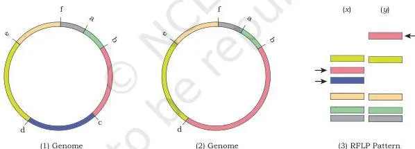
Figure 5.3 shows exactly this comparison. Genomes (1) and (2) share the same physical sites a–f except at site c: genome (1) carries restriction site c, while genome (2) has lost it. Digestion of genome (1) therefore gives two smaller unique bands, shown in lane (x); genome (2) gives one larger unique band, shown in lane (y). That one-lane difference is RFLP.
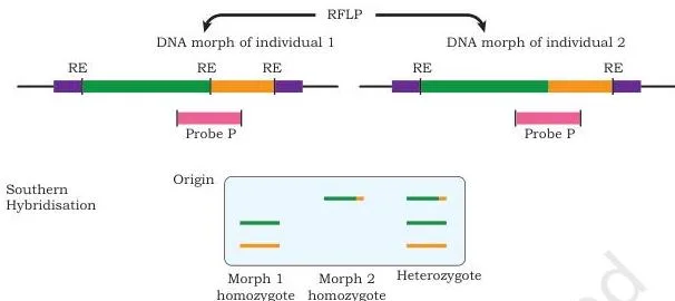
There is a scale problem the textbook flags: a restriction enzyme like EcoRI may cut a mammalian genome into lakhs of fragments, far more than a gel can resolve. The solution is Southern hybridisation — a specific labelled DNA probe, chosen between two RFLP sites, detects just the fragment of interest on the membrane (NCERT, p. 117).
Figure 5.4 shows the probe idea: probe P detects two DNA morphs when the DNA is cut by a certain restriction enzyme, so the same probe can reveal different-sized fragments in different individuals.
Simple Sequence Length Polymorphism (SSLP) uses length variants of repeat sequences as landmarks. Large genomes contain arrays of repeats of varying length — microsatellites and minisatellites — and these length variants serve as physical map features (NCERT, p. 118). These are the same repeat sequences introduced in Chapter 4 of this book, covered in our notes on the applications of recombinant DNA technology.
A Sequence Tagged Site (STS) is a unique DNA sequence of 200–500 bp that occurs once in a genome and whose location is known. Its presence in any DNA fragment can be demonstrated by PCR, which makes it a convenient location landmark. STS markers are often combined with restriction maps to improve resolution and the effectiveness of association mapping (NCERT, p. 118).
Three Generations of DNA Sequencing
Before cheap sequencing existed, full-genome sequencing was prohibitively expensive, so scientists first used maps to narrow attention to a small locus statistically associated with the phenotype of interest, and sequenced only that region (NCERT, p. 119). The three generations below are the story of removing that bottleneck.
First generation: chain termination
The first phase was a lengthy multi-step procedure (NCERT, p. 119):
- Separate chromosomes by Pulse Field Gel Electrophoresis (PFGE).
- Digest with restriction enzymes and ligate the fragments into high-capacity cloning vectors — BAC, YAC or PAC.
- Organise the overlapping clones into a minimum set that covers the organism’s DNA.
- Map the clones physically and sub-clone them into sequencing plasmids.
- Sequence by chain termination (the method from Class XI, section 12.9.1): a ladder of single-stranded DNA fragments, each terminating at a specific base that carries a specific fluorescent tag.
- Separate the fragments by capillary gel electrophoresis; a fluorescence detector reads each fragment as it passes.
- Read the output chromatogram — each peak is a base position, and the colour of the peak identifies the base.
Each capillary reads about 800–1000 bases per run, and one machine can run 96 capillaries in parallel — up to 96,000 bases per run (NCERT, p. 120). The drawbacks are equally clear: the process is time-consuming and labour-intensive, which makes full-genome sequencing prohibitively costly.
Second generation: Illumina bridge PCR
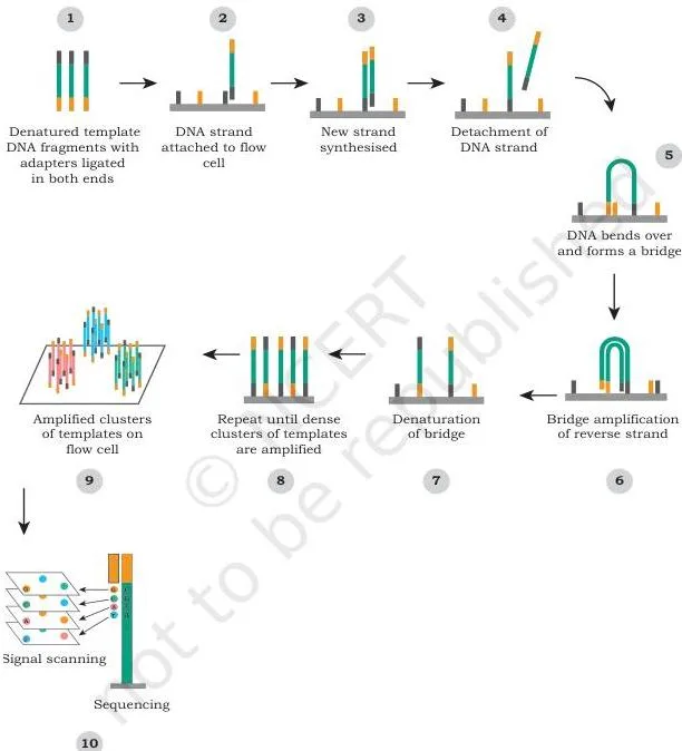
Next-generation sequencing is massively parallel — millions of sequencing reactions run in one machine. It removes the cloning and subcloning steps, lowers cost, and adds three advantages: a simple workflow, high data accuracy from high depth of coverage, and a broad range of applications (NCERT, p. 120). The pathway on an Illumina platform:
- Fragment the DNA to about 1–2 kb and attach small adaptors.
- On the flow cell (a glass slide), single-stranded oligonucleotides of 8–10 bases are already attached.
- The adaptors are complementary to these oligonucleotides, so DNA fragments attach to the flow cell.
- The adaptors act as primers for new-strand synthesis; the fragment folds into a bridge because its adaptors pair with the flow-cell oligonucleotides — hence bridge PCR amplification.
- Amplification produces a cluster of identical fragments at one location.
- A sequencing primer binds one adaptor, and fluorescently tagged dNTPs (dATP, dTTP, dGTP or dCTP) are added one base at a time — only one base type is incorporated at a time.
- An image records the fluorescence of every incorporated base, the tag is removed, and the next base is passed through; the final array of images reveals the sequences of millions of spots in parallel (NCERT, p. 122).
The trade-off is short reads — 75 to 300 bases — compared with first-generation reads.
Figure 5.5 maps this workflow: DNA fragments with adaptors attach to the flow cell, are amplified into clusters by bridge amplification, and are then read base-by-base as fluorescent images.
Third generation: nanopore sequencing
Nanopore sequencing reads bases by their effect on an electric current. Two proteins do the work: a DNA helicase, which captures and unwinds double-stranded DNA and pushes one strand through the pore, and a porin-like molecule assembled into a nanopore on a synthetic membrane (NCERT, p. 123).
An ionic current is maintained across the pore and monitored continuously. As each single-stranded base passes through, the pore interacts with it differently and disrupts the current in a base-specific way; by measuring those current signatures, the machine identifies the bases.
Figure 5.6 shows the arrangement: the yellow dots are ions flowing through the pore and generating the measured current; the helicase docks on the protein pore and drives one DNA strand through it. The sequence read in the diagram is ACGT.
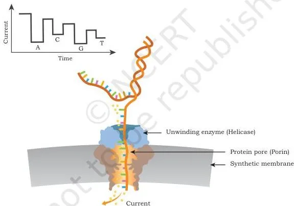
Nanopore sequencing offers rapid and simple sample processing, real-time display of results (useful even for field genotyping), and very long reads — up to about 1 Mb or more — at relatively low cost (NCERT, p. 124).
Why each generation displaced the previous one: the first generation was priced out of whole genomes by its labour and time costs. The second generation removed the bottleneck with massive parallelism and no cloning or subcloning — but delivered short reads. The third generation attacked the short-read problem with very long reads, real-time output and relatively low cost.
Every generation fixed the previous one’s most expensive weakness and accepted a new trade-off.
| Feature | First generation | Second generation (Illumina) | Third generation (nanopore) |
|---|---|---|---|
| Principle | Chain termination; capillary gel electrophoresis | Bridge PCR clusters; one fluorescent base at a time | Changes in ionic current as bases pass a nanopore |
| Read length | 800–1000 bases per capillary | 75–300 bases | Up to about 1 Mb or more |
| Parallelism | 96 capillaries per machine | Millions of reactions per machine | Single molecules read in real time |
| Workflow | Cloning, subcloning, capillary runs | No cloning/subcloning; simple workflow | Rapid, simple sample preparation |
| Cost and speed | Time-consuming, labour-intensive, costly | Lower cost; high depth of coverage | Relatively low cost; real-time results |
| Limitation | Prohibitive cost per base | Short reads | — |
Sequencing Variations: WGS, Targeted, RNA-seq, ChIP-seq and Metagenomics
Genome sequencing comes in multiple flavours, and each answers a different biological question (NCERT, p. 124):
| Variation | What it sequences | Question it answers |
|---|---|---|
| Whole Genome Sequencing (WGS) | The entire genome — first done for Haemophilus influenzae; human genome 1990–2003, now achievable in days | What is the complete genetic makeup? Which chemotherapy suits this cancer? |
| Targeted sequencing | Selected genes or genomic regions, usually isolated by PCR | Do specific regions carry mutations, insertions or deletions? |
| Clinical exome sequencing | Only genes known to be disease-associated (curated from databases such as OMIM and HGMD) | Cost-effective genetic diagnosis of known disease genes |
| ChIP-seq | DNA bound by a transcription regulator across the genome | Which target genes does this regulator control? |
| RNA-seq | cDNA synthesised from the total RNA of a sample | What is the global gene expression profile (transcriptome)? |
| Metagenomics | Total genetic material of a microbial community, without culturing | Who lives in this environment and what can their genes do? |
WGS was first achieved for the bacterium Haemophilus influenzae. The human genome project started in 1990 and the complete sequence was published in 2003 (NCERT, p. 124). WGS now helps create personalised treatment plans — for example, reading the variations in cancer cells can help a physician select the best chemotherapy.
Assembly comes in two modes: reference-based, in which the reads are assembled against an already sequenced, phylogenetically related reference genome, and de novo, in which no reference is used.
Targeted sequencing sequences only selected genes or genomic regions and uses a reference genome to assemble the new reads. It can compare the same small set of regions across genomes to identify variations such as mutations, insertions or deletions (NCERT, p. 125).
Clinical exome sequencing is the same strategy restricted to disease-associated genes curated from databases like OMIM and HGMD, and it is more cost-effective than whole genome sequencing.
ChIP-seq maps the genome-wide DNA binding sites of a transcription regulator. Since regulators control the expression of one or more genes, ChIP-seq reveals the regulator’s target genes across the whole genome.
RNA-seq profiles global gene expression: total RNA is extracted, cDNA is synthesised and sequenced with next-generation technology, and the reads are mapped back to genes — the count of reads mapping to a gene is proportional to its expression level (NCERT, p. 125).
Metagenomics studies the genomics of a community rather than a single organism. Total genetic material is obtained directly from the microorganisms living in an environment — members are not cultured or separated first (NCERT, p. 126).
- Applications span medical microbiology, agriculture and environmental microbiology.
- It reveals the diversity of microbial communities and how that diversity changes with the environment.
- It can identify novel genes or enzymes of industrial value — for example, microbes from high-temperature sulphur springs yield enzymes that stay functional at such high temperatures.
- It is used on gut microbes, throat microbes and more; viral metagenomics informs virus-host interaction, epidemiology and virus evolution.
- A metagenomics sample contains multiple genomes, so its data analysis needs a different set of computing algorithms.
Genome Engineering: Transposons and the CRISPR-Cas9 Scissors
Genome engineering modifies a genome — usually to introduce or remove one or more genes. The stated goal is to introduce a new functionality or to modify (or remove) an existing functionality of the organism (NCERT, p. 126). The chapter gives two routes: transposons and CRISPR-Cas9.
Transposons: knock-out and knock-in
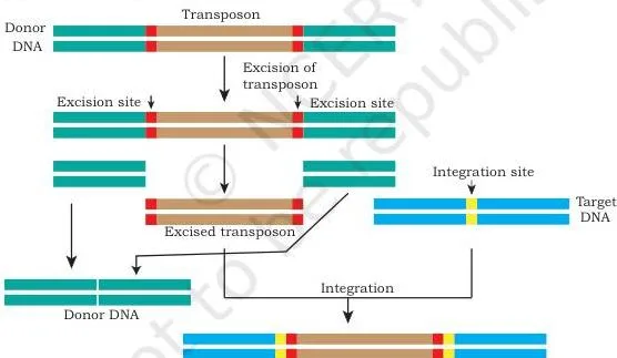
Transposons, or “jumping genes”, are DNA sequences that move from one location to another on the genome, and they are found in almost all organisms, prokaryotic and eukaryotic. DNA transposons move by a cut-and-paste mechanism — excised from one location and integrated elsewhere (NCERT, p. 127).
- Knock-out: the transposon is engineered to recognise a specific sequence in the target gene and insert there. Insertion disrupts the coding frame, so the gene can no longer produce its original transcript and its product disappears — insertional inactivation.
- Knock-in: when insertion at a site adds DNA sequence that was not present there, the transposon can bring in a functional gene.
- Use: generating animal and plant models to understand the molecular basis of disease and to develop new drugs (NCERT, p. 128).
Figure 5.7 shows the strategy: the jumping element is excised from its original position, moves, and is pasted into the target gene, where it disrupts the coding frame so the transcript can no longer be made.
CRISPR-Cas9: the guide-RNA scissors
CRISPR-Cas9 is a biotechnological repurposing of a natural genome-editing system present in bacteria. In nature, bacteria use it to memorise the DNA signatures of past viral attacks, so that any later infection carrying a matching DNA signature is countered or destroyed (NCERT, p. 128).
For editing, a guide RNA is designed and produced in the cell together with the Cas9 endonuclease. One part of the guide RNA is complementary to the DNA region to be edited; another part binds Cas9. Once the complex assembles at the target, Cas9 introduces a double-strand break.
The break is then repaired by template-based homologous DNA repair: a modified, edited template carrying the desired changes is provided, and the repaired DNA ends up with the edited sequence.
Figure 5.8 shows both outcomes of the double-strand break. Path one: deletion or insertion of DNA at the break creates a gene knock-out. Path two: a desired mutant copy is introduced at the break site and, in the presence of that mutant template, homologous recombination places the mutations at exactly that spot — a precise edit, not a random one.
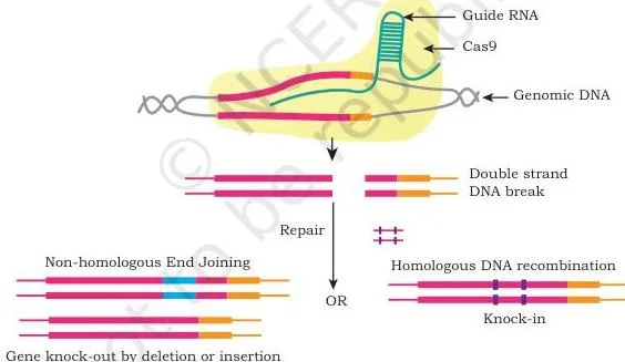
Why does CRISPR need a template? Without a template, the cell repairs the break imprecisely — DNA is deleted or inserted at the break, which is exactly how the knock-out arises. With an edited template, homologous recombination copies the desired change faithfully.
In 2020, the Nobel Prize in Chemistry went to Emmanuelle Charpentier and Jennifer A. Doudna for discovering the CRISPR-Cas9 genetic scissors (NCERT, p. 129). Working on Streptococcus pyogenes in 2011, Charpentier discovered tracrRNA, a molecule in the CRISPR-Cas system; together with Doudna she showed that CRISPR could be directed to cut DNA at chosen target sequences using Cas9.
The cell’s own repair machinery then adds, deletes or changes DNA, which is what makes the tool precise.
From Sequence to Biology: Structural, Functional and Comparative Genomics
Next-generation projects generate large volumes of data, and the chapter opens this section with the computational layer before the three biological branches. Computational genomics uses high-performance computing clusters and workstations to analyse sequencing data.
Homology search and gene annotation (assigning functional value) identify common genes, and tools such as BLAST, ClustalW and Phylip compare sequences across multiple genomes to understand evolutionary relationships (NCERT, p. 130). General-purpose GPU and CUDA programming accelerate these analyses.
The three branches are best compared side by side:
| Branch | Focus | What it studies / tools |
|---|---|---|
| Structural genomics | 3D structure of every protein encoded by a genome; plus the physical organisation of the whole genome | Searching for new protein folds; chromosome and nucleosome status; large structural changes between related species — for example, how genes common to mice and humans are redistributed across different chromosomes |
| Functional genomics | How the physiological information encoded in the genome is executed | Uses RNA-seq, ChIP-seq and metagenomics to connect genome data to the physiological and pathological state of a cell |
| Comparative genomics | Comparison of genes and genomes across species or among individuals of the same species | Genome annotation of new sequences; identifies the common core genome and species-unique genes; presence or absence of functional molecules; a starting point for genome-based taxonomy and phylogenetic study |
The chapter also records the Indian infrastructure behind this work: the Department of Biotechnology (Ministry of Science and Technology, Government of India) has established three National Genomics Core facilities — at the Centre for DNA Fingerprinting and Diagnostics (Hyderabad), the National Institute of Biomedical Genomics (Kalyani) and the University of Allahabad (Prayagraj) — so that Indian scientists and entrepreneurs can carry out genomic projects locally (NCERT, pp. 130–131).
Protein Engineering: Four Engineered Proteins to Remember
The principle comes first: identify the critical amino acids responsible for the desired trait, then modify their codon sequences by point mutations so the amino acid is replaced. The engineered protein then gains an extended property — greater stability at elevated temperature, changed pH, or in the presence of salts or organic solvents, or even a new function (NCERT, p. 132).
The chapter’s four worked applications are summarised below, with the textbook details following.
| Protein | Problem / goal | Engineering change | Outcome |
|---|---|---|---|
| Subtilisin | Bleach oxidises Met 222 and reduces the enzyme’s action | Replace the Met 222 codon with an Ala codon by site-directed mutagenesis | Bleach-stable detergent enzyme |
| 6-His-tag | Recombinant protein difficult to purify | Fuse DNA for six consecutive histidines to the gene of interest | Tagged protein binds nickel, zinc and cobalt for affinity purification |
| GFP | Need to see where a protein sits inside a cell | Fuse the GFP gene from Aequorea victoria to the gene of interest | Chimeric protein glows green under UV; localisation seen by microscopy |
| Recombinant immunotoxin | Kill cancer cells selectively | Fuse an scFv (VH and VL joined by a flexible linker) to a toxin | Binds the cancer antigen, is internalised, and the toxin kills the cell |
1. Subtilisin: a bleach-stable detergent enzyme
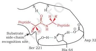
Subtilisin is a proteolytic enzyme added to detergents to hydrolyse the protein component of dirt. Its catalytic triad is Ser 221, His 64 and Asp 32. In the presence of bleach, the adjacent Met 222 is oxidised, which reduces the enzyme’s action. Replacing the Met 222 codon with an Ala codon by site-directed mutagenesis makes the engineered protein stable even in bleach (NCERT, p. 132).
Figure 5.9 shows the catalytic triad — the three active-site residues Ser 221, His 64 and Asp 32 that carry out the catalysis.
2. 6-His-tag: one-step protein purification
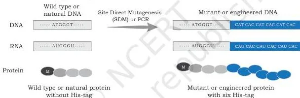
A 6-His-tag is a peptide of six consecutive histidines that binds metal ions — nickel, zinc and cobalt — with great affinity at mildly alkaline pH. DNA encoding the tag is fused to the recombinant gene of interest.
During affinity chromatography, the tagged protein is immobilised by the metal ions in the agarose gel while other proteins wash away; the tagged protein is then eluted with an elution buffer (NCERT, p. 133). Figure 5.10 shows the payoff: a 6-His-tagged engineered protein is easily and efficiently purified on a nickel-ion column.
3. GFP: tracking a protein’s location
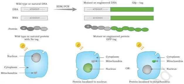
The gene for green fluorescent protein (GFP) comes from the jellyfish Aequorea victoria. When it is fused to the DNA sequence of interest, the resulting chimeric DNA encodes an engineered protein that glows green under UV light, revealing its location inside the cell (NCERT, p. 133).
Figure 5.11 shows a GFP-tagged protein localised to the nucleus: under UV light it appears green, and epifluorescence or confocal microscopy reveals which cell region it occupies.
4. Recombinant immunotoxin: selective cell killing
A recombinant immunotoxin combines the selectivity of an antibody with the cell-killing potency of a toxin. The antibody part is a single-chain variable fragment (scFv): the variable regions of the heavy (VH) and light (VL) chains, joined by a short flexible peptide linker.
Because it is encoded by a single gene, the scFv is a single polypeptide chain and can be produced conveniently in bacteria (NCERT, p. 134).
- Design: an scFv that binds a specific antigen on cancer cells is fused to a toxin such as Pseudomonas exotoxin A, diphtheria toxin or ricin, using a linker that lets both parts fold and act.
- Mechanism: the antibody part binds the cancer cell’s surface antigen; the whole protein is internalised by endocytosis; the toxin is released from the endosome and kills the cell.
- Construction sequence (from the textbook diagram): natural antibody → scFv with linker → DNA of light chain, heavy chain and toxin joined by linkers → finished recombinant immunotoxin → binding to a cell-surface receptor → internalisation leading to cell death.
Box 3: humanised monoclonal antibodies
Monoclonal antibodies produced by mouse hybridoma technology (Chapter 4 of this book) bind their targets precisely, but the human immune system recognises them as foreign and raises an anti-mouse immune response.
Protein engineering solves this at the DNA level: the part of the mouse antibody involved in antigen binding is identified, and its coding DNA is transferred into a human antibody gene. The resulting humanised antibody is often considered self, so it has good immune acceptance when administered therapeutically (NCERT, p. 135).
Key Terms of Genome Engineering, Defined
One pass through the chapter’s vocabulary — every term below appears in the textbook, with the chapter’s own example as the memory hook:
| Term | Meaning | Example from the chapter |
|---|---|---|
| Genome | Complete genetic information present in the cell | Prokaryote: nucleoid + plasmid; eukaryote: nuclear chromosomes + organelles |
| Genetic map | Loci arranged by recombination-based distances | cM distances from offspring phenotype frequencies |
| Physical map | Locations identified by DNA-based features | Restriction maps, SSLP, STS |
| Map unit / centimorgan | 1 map unit = 1% recombinants | 15% recombinants → 15 cM |
| RFLP | Variation in fragment length when DNA is cut by the same restriction enzyme | EcoRI digest giving different bands in two individuals |
| SSLP | Length variants of repeat sequences | Microsatellite and minisatellite repeats |
| STS | Unique 200–500 bp sequence, single copy, known location | Detectable by PCR |
| Southern hybridisation | Probe-based detection of specific DNA fragments | Probe P detects two DNA morphs after restriction digestion |
| Whole genome sequencing | Sequencing the entire genome | First done for Haemophilus influenzae; human 1990–2003 |
| Reference-based vs de novo sequencing | Assembly with or without a reference genome | Human reads assembled against a reference vs assembling a new species |
| Targeted sequencing | Sequencing selected genes or regions | PCR-isolated regions; finds mutations, insertions, deletions |
| Clinical exome sequencing | Sequencing disease-associated genes | Genes curated from databases like OMIM and HGMD |
| ChIP-seq | Maps genome-wide DNA-binding sites of a transcription regulator | Reveals the regulator’s target genes |
| RNA-seq | Global expression (transcriptome) profiling | Read count per gene is proportional to expression level |
| Metagenomics | Direct sequencing of the total genetic material of a community | Gut microbes; enzymes from sulphur springs |
| Transposon | Moving DNA element, “jumping gene”, cut-and-paste movement | DNA transposons in almost all organisms |
| Knock-out | Gene inactivated by insertion | Transposon insertion disrupts the coding frame |
| Knock-in | Adding a functional gene by insertion | Transposon adds absent DNA sequence at a locus |
| CRISPR-Cas9 | Guide RNA + Cas9 endonuclease editing system | Double-strand break + template-guided homologous repair |
| Guide RNA | RNA that positions Cas9 at the target | One part complementary to target DNA, other part binds Cas9 |
| Structural genomics | 3D structures of proteins; whole-genome physical organisation | New protein folds; mouse vs human gene redistribution |
| Functional genomics | How genome information is executed in cells | RNA-seq, ChIP-seq, metagenomics |
| Comparative genomics | Comparing genomes across species or individuals | Core genome vs species-unique genes |
| 6-His-tag | Six-histidine peptide used for purification | Binds nickel, zinc, cobalt at mildly alkaline pH |
| GFP | Green fluorescent protein from Aequorea victoria | Fusion tag makes proteins glow green under UV |
| Recombinant immunotoxin | scFv fused to a toxin | Pseudomonas exotoxin A, diphtheria toxin, ricin |
| Humanised monoclonal antibody | Mouse antigen-binding part transferred into a human antibody | Accepted as self; good therapeutic acceptance |
Key Units and Quantitative Rules of Chapter 5
Chapter 5 has no algebraic formulas, but it carries specific numbers and proportional rules. These are the quantitative facts to be able to recall cold:
| Rule / value | Statement | Where it appears |
|---|---|---|
| 1 map unit | = 1% observed recombinants; expressed as centimorgan (cM) | Genetic mapping, NCERT p. 116 |
| Recombination vs distance | Chances of loci separating by recombination are directly proportional to their distance | Genetic mapping, NCERT p. 116 |
| Circular DNA cuts | \(n\) cuts → \(n\) fragments | Restriction mapping, NCERT p. 116 |
| Linear DNA cuts | \(n\) cuts → \(n+1\) fragments | Restriction mapping, NCERT p. 116 |
| STS size | Unique 200–500 bp, single copy, PCR-demonstrable | Physical mapping, NCERT p. 118 |
| First-generation reads | 800–1000 bases per capillary; 96 capillaries → up to 96,000 bases per run | NCERT p. 120 |
| Illumina numbers | Reads of 75–300 bases; flow-cell oligonucleotides 8–10 bases; fragments ~1–2 kb | NCERT pp. 120–122 |
| Nanopore reads | Up to about 1 Mb or more | NCERT p. 124 |
| Human Genome Project | Started 1990; complete sequence published 2003 | NCERT p. 124 |
| First-generation cloning vectors | BAC, YAC, PAC | NCERT p. 119 |
The textbook’s own exercises lean on several of these numbers: Q3’s BamHI digest applies the fragment-count rule, Q5, Q6 and Q8 ask about sequencing technology and its capacities, and Q9 asks for the variations of next-generation sequencing (NCERT, pp. 138–139).
Worked Examples: Restriction Maps, Genetic Distances and Sequencing Runs
Example A: Deduce a restriction map from single and double digests
Method: use the linear-DNA rule — one cut produces two fragments, and the fragment lengths must add up to the full molecule length.
Step 1: A \(6.0\ \text{kb}\) linear DNA digested with BamHI gives bands of \(4.0\ \text{kb}\) and \(2.0\ \text{kb}\).
Because there are exactly two bands, there is one BamHI site, \(2.0\ \text{kb}\) from the left end.
Step 2: Digestion with HindIII gives \(3.5\ \text{kb}\) and \(2.5\ \text{kb}\).
There is one HindIII site, \(3.5\ \text{kb}\) from the left end.
Step 3: Predict the double-digest fragments for this arrangement — BamHI at \(2.0\ \text{kb}\) and HindIII at \(3.5\ \text{kb}\):
\[ 2.0\ \text{kb};\quad 1.5\ \text{kb};\quad 2.5\ \text{kb} \]
\[ 2.0 + 1.5 + 2.5 = 6.0\ \text{kb} \]
Step 4: Test the alternative — a HindIII site \(3.5\ \text{kb}\) from the right end, i.e.
at \(2.5\ \text{kb}\) from the left.
With BamHI at \(2.0\ \text{kb}\), the double digest would give \(2.0\ \text{kb}\), \(0.5\ \text{kb}\) and \(3.5\ \text{kb}\), which does not match the observed bands of \(2.0\), \(1.5\) and \(2.5\ \text{kb}\).
Final answer: the BamHI site lies \(2.0\ \text{kb}\) and the HindIII site \(3.5\ \text{kb}\) from the left end of the \(6.0\ \text{kb}\) molecule.
Example B: Convert a recombination frequency into a genetic distance
Method: use the definition of the map unit — 1 map unit = 1% recombinants, written in centimorgans (cM).
Step 1: A test cross of 240 offspring shows 204 parental types and 36 recombinants.
The recombination frequency is:
\[ \frac{36}{240} = 0.15 = 15\% \]
Step 2: Convert to map units: \(15\%\) recombinants means the loci are \(15\ \text{map units}\) apart, i.e.
\(15\ \text{cM}\).
Step 3: Interpret the result: recombination frequency is directly proportional to distance, so a smaller recombinant fraction would mean the loci are closer.
Here, \(15\ \text{cM}\) apart is the genetic distance between the two loci.
Final answer: the genetic distance is \(15\ \text{cM}\).
Example C: Estimate first-generation sequencing runs for a bacterial genome
Method: divide the total genome length by the bases read per run, then round up to a whole number of runs.
This estimate assumes \(1\times\) coverage — one read per base of the genome.
Step 1: Bases per run = 96 capillaries \( \times \) 800 bases per capillary:
\[ 96 \times 800 = 76{,}800\ \text{bases per run} \]
- Step 1: Genome length = \(4.8\ \text{Mb} = 4{,}800{,}000\ \text{bp}\).
- Step 2: Number of runs needed:
\[ \frac{4{,}800{,}000}{76{,}800} = 62.5 \]
Step 4: A fraction of a run is impossible, so round up: 62 runs cover only part of the genome, so the 63rd run is required.
Final answer: about 63 runs at \(1\times\) coverage.
Closing point: real projects sequence at higher depth of coverage — the textbook names high depth of coverage as a next-generation advantage — so 63 runs is a bare lower bound.
This economics is precisely why first-generation sequencing gave way to next-generation machines.
Common Mistakes Students Make in This Chapter
Eight chapter-specific confusions, each with the correction and a quick way to check yourself:
| Students write… | Correct is… | How to check your answer |
|---|---|---|
| “One cut in circular DNA gives two fragments.” | A single cut opens the circle, giving one fragment; two cuts give two fragments. Circular: \(n\) cuts → \(n\) fragments. | Draw the circle and cut it once — you get one piece. |
| “Genetic distance in cM is a physical distance in base pairs.” | cM is a recombination-based relative distance; \(1\ \text{cM} = 1\%\) recombinants. Base-pair positions belong to physical maps. | Check the unit’s origin: cM comes from offspring data, not from DNA landmarks. |
| “Cas9 finds the target by itself.” | The guide RNA positions Cas9: one part of it is complementary to the target DNA, and the other part binds Cas9. | Trace the complex: guide RNA + target DNA + Cas9 → double-strand break. |
| “CRISPR always knocks the gene out.” | Without a template, deletion or insertion at the break creates a knock-out. With an edited template, homologous recombination makes precise edits. | Ask: was a mutant template provided for repair? |
| “STS and SSLP are the same kind of repeat landmark.” | STS is a unique 200–500 bp single-copy sequence; SSLP is a length variant of microsatellite/minisatellite repeats. | Compare the definitions: unique sequence vs repeat length. |
| “Metagenomics cultures each microbe separately first.” | Total genetic material is extracted directly from the community sample, without culturing organisms individually. | Look for the phrase “total genetic material directly obtained”. |
| “The 6-His-tag makes a protein glow under UV.” | The 6-His-tag is for metal-affinity purification (binds nickel, zinc, cobalt). GFP is the fluorescent tag. | Match the tag to its application: purification vs localisation. |
| “To survive bleach, subtilisin’s catalytic triad is replaced.” | The triad (Ser 221, His 64, Asp 32) stays intact; bleach oxidises Met 222, and it is Met 222 that is replaced by Ala. | Name the residues: the triad is conserved; Met 222 → Ala. |
Exam Notes: Structuring Complete Answers for the Textbook Exercises
This section is structure guidance for the 21 exercises on pages 138–139 — it is not model answers. Read the question stem, then build your answer in the shape described below.
Q1 — genome
Give the definition first (complete genetic information present in the cell), then contrast prokaryotes and eukaryotes: nucleoid plus plasmid against nuclear chromosomes plus organelles such as mitochondria and plastids.
Q2, Q3, Q4, Q7 — mapping cluster
Always give the basis (recombination vs DNA landmarks), the unit (cM vs physical sites), the map features and the resolution. For Q3, state that a BamHI digest builds a restriction (physical) map, then give its application — detecting the gain or loss of restriction sites, such as comparing family members for disease association.
For Q4 and Q7, build the answer around STS as a unique 200–500 bp single-copy landmark demonstrable by PCR, and around the physical map’s DNA-based features.
Q5, Q6, Q8, Q9, Q10 — sequencing cluster
Arrange answers chronologically. First describe the first-generation workflow (PFGE, cloning into BAC/YAC/PAC, chain termination, capillary electrophoresis, chromatogram), then the problems it created (time, labour, cost). Next explain how massively parallel sequencing solved them — no cloning or subcloning, lower cost, high depth of coverage, with short reads as the trade-off.
Then cover the third generation (helicase + porin-like pore, ionic current changes, long reads, real-time results). For Q9, list the variations of next-generation sequencing (WGS, targeted, clinical exome; ChIP-seq and RNA-seq as advanced applications); for Q10, give each advanced application’s purpose — ChIP-seq for regulator binding sites, RNA-seq for expression, and the community-level uses of metagenomics.
Q11 — metagenomics
Define metagenomics as the study of total genetic material obtained directly from a microbial community without culturing, then list its named applications: gut and throat microbes, novel industrial enzymes from extreme environments such as high-temperature sulphur springs, and understanding virus-host interaction, epidemiology and virus evolution.
Q12, Q13, Q14 — genome engineering
State the goals first (introduce or remove genes; add a new functionality or modify/remove an existing one), then the mechanism: transposon cut-and-paste (knock-out by insertional inactivation, knock-in by adding a sequence) or CRISPR (guide RNA + Cas9 → double-strand break → template-guided homologous repair).
Q13 is the one honest gap in the chapter: the textbook poses the question, but a detailed answer must draw on the genome-engineering goals plus the gene-expression concepts from earlier chapters — those are covered in our applications of recombinant DNA technology notes.
Q15 — the three genomics
Define each branch with one anchoring tool or example: structural genomics (new protein folds; chromosome and nucleosome organisation), functional genomics (RNA-seq, ChIP-seq, metagenomics), and comparative genomics (core genome, species-unique genes, genome-based taxonomy).
Q16–Q19 — protein engineering
Present each application as problem → engineering change → outcome. Subtilisin: Met 222 → Ala for bleach stability. 6-His-tag (Q17): methodology — fuse the tag, run affinity chromatography on a metal column, wash away other proteins, elute with elution buffer. GFP (Q18): fuse the GFP gene from Aequorea victoria, then detect the green fluorescence by epifluorescence or confocal microscopy.
Immunotoxin (Q19): why it is needed (selective cancer-cell killing), how it is built (scFv linked to a toxin such as Pseudomonas exotoxin A, diphtheria toxin or ricin), and its mechanism (bind → internalise by endocytosis → toxin released from the endosome → cell death).
Q20, Q21 — assertion-reason questions
Test the assertion alone, test the reason alone, then decide whether the reason actually explains the assertion. The four options follow directly from that three-step check.
A general rule for any “explain in detail” exercise: write state → mechanism/steps → outcome, in that order. A complete answer earns its completeness by naming the components and then connecting them, not by listing words.
Revision Summary: Chapter 5 in One Page
One-line triggers for the night before:
| Chapter section | Remember this |
|---|---|
| Genome (NCERT p. 113) | Prokaryotes: nucleoid + plasmid. Eukaryotes: nuclear chromosomes + organelles (mitochondria, plastids). |
| Genetic vs physical maps (pp. 115–116) | Genetic = recombination distances (cM); physical = DNA landmarks (restriction sites, SSLP, STS). |
| Fragment rule (p. 116) | Circular: \(n\) cuts → \(n\) fragments. Linear: \(n\) cuts → \(n+1\) fragments. |
| Sequencing generations (pp. 119–124) | Chain termination (capillary) → Illumina bridge PCR (clusters, short reads) → nanopore (ionic current, long reads). |
| Sequencing variations (pp. 124–126) | WGS, targeted/exome, ChIP-seq, RNA-seq, metagenomics — each answers a different question. |
| Genome engineering (pp. 126–129) | Transposon: cut-and-paste → knock-out or knock-in. CRISPR: guide RNA + Cas9 → double-strand break → template repair. |
| Genomics branches (pp. 130–132) | Structural (3D structures, genome organisation), functional (execution of information), comparative (core genome). |
| Protein engineering (pp. 132–135) | Four applications: subtilisin, 6-His-tag, GFP, immunotoxin (+ humanised antibodies). |
Mnemonic for the four protein applications: “Subtilisin scrubs, His-tag grabs, GFP glows, Immunotoxin kills.”
Six-point self-check — can you:
- define 1 cM in one sentence?
- apply the \(n\)-cut fragment rule to circular and linear DNA?
- tell STS from SSLP?
- contrast reference-based with de novo WGS?
- distinguish knock-out, knock-in and precise CRISPR editing?
- name all four protein-engineering applications with one detail each?
Frequently Asked Questions
What is the difference between genetic mapping and physical mapping?
Genetic mapping measures relative distance between loci by recombination frequency, using crossover analysis of loci with well-known phenotypes; its unit is the map unit or centimorgan (1 unit = 1% recombinants). Physical mapping identifies locations using DNA-based landmarks — restriction enzyme sites, SSLP and STS — and gives high resolution.
Because few well-known phenotypic loci exist, genetic maps stay coarsely grained, while physical maps can be packed densely enough for fine mapping of new phenotypes.
How does bridge PCR amplification work in Illumina sequencing?
DNA is fragmented to about 1–2 kb and given adaptors that are complementary to the 8–10 base oligonucleotides fixed on a flow cell. The fragments attach to the flow cell, and the adaptors act as primers for new-strand synthesis; the fragment folds into a bridge because its adaptors pair with the flow-cell oligonucleotides.
Amplification then produces a cluster of identical fragments at one location, ready for one-base-at-a-time fluorescent sequencing.
What is the difference between knocking out and knocking in a gene with a transposon?
A knock-out happens when the transposon inserts inside a gene and disrupts its coding frame, so the original transcript can no longer be produced — insertional inactivation. A knock-in happens when the insertion adds DNA sequence that was not present at the locus, bringing in a functional gene.
Both are used to generate animal and plant models for studying the molecular basis of disease and developing new drugs.
How does nanopore sequencing identify DNA bases?
A DNA helicase unwinds double-stranded DNA and pushes one strand through a porin-like nanopore on a synthetic membrane, while an ionic current is maintained across the pore. Each base passing through disrupts that current in a specific, characteristic way, and measuring those current signatures identifies the bases. The sequence read in the textbook diagram is ACGT.
Why did next generation sequencing replace first generation sequencing?
First-generation chain-termination sequencing was time-consuming, labour-intensive and costly, and it required cloning and subcloning. Next-generation methods run millions of sequencing reactions in parallel in one machine, remove the cloning and subcloning steps, and provide high data accuracy through high depth of coverage at lower cost.
The trade-off is short reads of 75–300 bases, compared with the 800–1000 base reads of first-generation capillary sequencing.
What are the four applications of protein engineering covered in this chapter?
Subtilisin made bleach-stable by replacing Met 222 with Ala; the 6-His-tag for metal-affinity purification on nickel-ion columns; GFP tagging (from Aequorea victoria) to track a protein’s location in the cell by UV fluorescence; and recombinant immunotoxins — an scFv antibody fragment fused to a toxin such as Pseudomonas exotoxin A, diphtheria toxin or ricin — that kill cancer cells selectively.
Reference: NCERT Class 12 Biotechnology textbook, chapter Genome Technology and Engineering.
Explore Class 12 Biotechnology Notes
- Class 12 Biotechnology Notes
- Class 12 CBSE Notes
- CBSE Notes for Classes 1 to 12
- Previous: Applications of Recombinant DNA Technology
- Next: Plant Tissue Culture
Class 12 Biotechnology on LearnCBSE:
Related chapters:
- Recombinant DNA Technology notes
- Host–Vector System notes
- Gene Cloning notes