
These Graphs and Charts Class 12 notes give you a complete, exam-ready revision of Chapter 4 of the NCERT Computerised Accounting System textbook — every definition, chart element, Excel step and limit you need in one place. They follow the 2026-27 session (Rationalised NCERT edition).
Read them top to bottom for a full revision, or jump through the table of contents to the section you need. The worked example builds a bar chart and a pie chart from a fresh dataset with every calculation shown, and the quick-revision section at the end compresses the whole chapter into tables you can scan before a test.
What This Chapter Covers: From Data to Decisions
The chapter sets two learning objectives (NCERT, p. 105): you should be able to represent accounting data graphically through Excel, and use accounting data for graphical representation in business communication. These notes are part of our Class 12 Accountancy notes collection, and this chapter assumes the spreadsheet basics from the previous chapter of the same book: worksheets, rows, columns and the Ribbon.
To teach chart-making, the book follows one running example — ABC Manufacturing Company Ltd — whose worksheet carries the quarterly sales (Qtr1 to Qtr4) of six products: toothpaste, toothbrush, hair oil, shampoo, toilet soap and bath soap. Row 11 holds quarter-wise totals, column G holds product-wise totals, and cell G11 holds the grand total for the year.
You do not need to memorise these figures; you need to remember the shape of the worksheet, because every chart in the chapter is built from a small part of it.
The motivation is simple: a mass of raw data is hard to understand, and the book quotes the saying that “a picture is worth more than a thousand words” (NCERT, p. 105). A chart compresses many numbers into one visual that a reader absorbs in seconds — which is exactly why managers use charts before making business decisions.
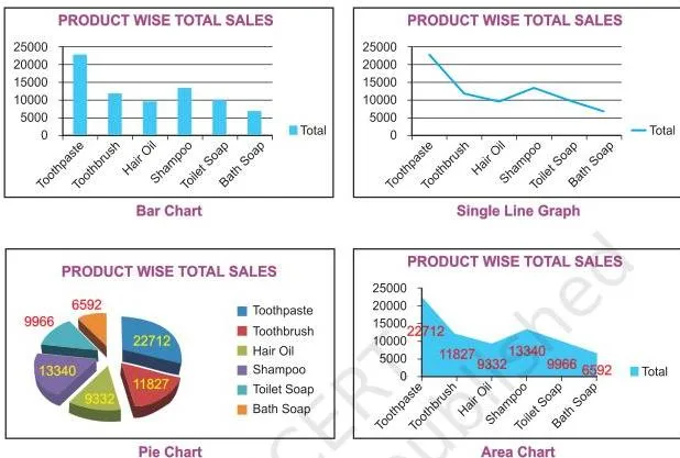
Figure 4.1 shows the spread of graph and chart forms Excel can prepare using the commands or standard tools on the toolbar — line, column, bar, pie, doughnut, radar and 3-D forms are different chart types that Excel can prepare. The rest of this page teaches you each of those forms, starting with the definitions.
If you want to verify any detail against the official text, the NCERT chapter is on the NCERT website.
Core Definitions: Graph, Pie Chart and Bar Diagram
- Graph — a pictorial representation of data that carries at least a two-dimensional relationship (NCERT, p. 105). That two-dimensional quality is why every graph has at least two axes: the X-axis, usually horizontal, and the Y-axis, usually vertical.
- Single-line and multi-line graphs — a graph may be a single line, or several lines in one figure. To keep a multi-line graph readable, different line types, shapes and shades of colour distinguish one line from another (NCERT, p. 105).
- Pie chart — represents the multiple sub-groups of a single variable: it divides one whole into its parts (NCERT, p. 105).
- Bar diagram — depicts two or more variables: it lines up separate values for comparison (NCERT, p. 105).
Keep the pie-versus-bar contrast clear: a pie divides one whole into shares, while a bar diagram compares separate values. If your question is “what fraction of one total?” it is pie material; if it is “how do these numbers compare?” it is bar material.
Everything else in the chapter — axes, series, legends, formatting — is detail layered on top of these two ideas.
The Elements of an Excel Chart: Chart Area, Axes, Series and More
To read any chart — or to find any Excel option later — you first need the element names the book uses (NCERT, pp. 108-109). Figure 4.6 shows them on a sample chart.
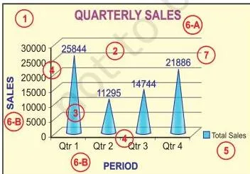
- Chart area — the entire chart, including all its elements.
- Plot area — the region in which the data is drawn. In a 2-D chart it is bounded by the X and Y axes; in a 3-D chart it is bounded by the X, Y and Z axes.
- Data points, data markers and data series — an individual value plotted in a chart is a data point, shown as a data marker (a bar, column, line, pie slice or other shape). Markers of the same colour form a data series — related data points plotted together. Each series has a unique colour or pattern, and a chart may hold more than one series.
- Horizontal (category) and vertical (value) axes — the X-axis is usually the horizontal line containing categories (independent values); the Y-axis is usually the vertical line containing data (dependent values).
- Legend — the identifier that shows which colour or pattern belongs to which series or category.
- Chart and axes titles — descriptive text naming the chart and each axis.
- Data labels — additional information attached to a data marker that identifies the detail of a data point in a series.
Some of these elements appear by default when Excel draws a chart; others are added only when you need them, and every element’s format or display can be changed (NCERT, p. 109). That is why the same chart can look plain in five minutes and polished in ten.
Chart Terminology at a Glance
| Term | Meaning in plain words | Where it matters |
|---|---|---|
| Graph | Picture of data with at least a two-dimensional (two-axis) relationship | Foundation of every chart in the chapter |
| Chart | Excel’s name for graphs and diagrams; in Excel, charts include graphs | You build both through Chart Tools |
| Single-line graph | One line plots one series | Trend of one series over time |
| Multi-line graph | Several lines, told apart by line type, shape or shade of colour | Comparing two or more series |
| Pie chart | Sub-groups of a single variable shown as shares of a whole | One series, at most seven categories |
| Bar diagram | Two or more variables shown as separate bars for comparison | Comparing absolute values |
| Chart area | The entire chart, all elements included | Selecting and moving the whole chart |
| Plot area | Region bounded by X and Y axes (2-D) or X, Y and Z (3-D) | Where data is actually drawn |
| Data point | One individual value plotted in the chart | The smallest unit of chart data |
| Data marker | The visual shape of a data point: bar, column, line, pie slice, etc. | The bars, columns and slices you see |
| Data series | Related data points of one colour or pattern | Each series gets its own legend entry |
| Legend | Identifier of each series or category in the chart | Tells you which colour means which series |
| Category axis (X) | Horizontal axis holding independent values or categories | Products, months and quarters sit here |
| Value axis (Y) | Vertical axis holding dependent (derived) values | Rupee amounts and counts sit here |
| Depth axis (Z) | Third axis of a 3-D chart, also called the series axis | Plots data along the depth of the chart |
| Origin (O) | Intersection of the X and Y axes | Positive values right/up; negative values left/down |
| Data label | Additional information about a data marker | Shows the exact value on a bar or slice |
| Gridline | Optional helper lines in the plot area that make values easier to estimate | Excel lets you display or hide them |
| Doughnut chart | Parts-to-whole with more than one series, one ring per series | Hard to read; prefer a stacked column or bar |
| Radar chart | Compares the aggregate values of several data series | Has no horizontal (category) axis |
Rule of thumb for the whole chapter: pie = parts of one whole; bar = compare separate values; line = trend over time.
Creating a Chart in Two Steps: Enter Data, Then Choose a Chart
The short route to Excel in the book is: Start icon → Programs → MS Excel 2007, which opens a blank workbook with the Ribbon at the top; then click the Insert tab to get the chart tools (NCERT, p. 107). With the workbook open, chart creation is exactly two steps.
- Step 1 — Enter the data with proper row and column titles. In the chapter’s example, product names are rows, the four quarters are columns, row 11 gives quarter-wise totals, column G gives product-wise totals, and cell G11 gives the grand total.
- Step 2 — Select the data you want to plot and choose a chart type from the Ribbon. Two common selections:
- Step 2a — bar chart of product totals: select the product names together with the product-wise totals (two consecutive columns) and insert a bar chart (NCERT, p. 107).
- Step 2b — column chart of quarter totals: reorganise the data so the quarters become the categories, then chart the quarter-wise totals; this produces the chart in Figure 4.5 (NCERT, p. 108).
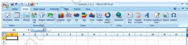
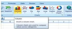
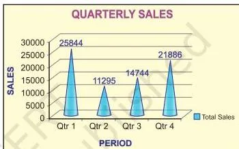
Figure 4.2 shows where the chart commands sit on the Ribbon and toolbar, and Figure 4.3 shows the chart tools that appear after clicking the Insert tab. Figure 4.5 shows the result of Step 2b: total sales for each quarter, with quarters now as the categories.
The layout rule that makes any chart correct: keep the labels column next to the values column. For a pie chart the book is explicit — you must select data from two consecutive columns only, labels plus values (NCERT, p. 114). The same tidy layout makes every other chart safer too.
Totals and Pie Percentages: The Chapter’s Two Calculations
The textbook prints no formula boxes in this chapter, but two calculations drive every chart you build (NCERT, pp. 107-108, 113-114). Making them explicit lets you check any chart by hand, exactly as the worked example below does.
Calculation 1 — Totals (unit: Rs)
\[ \text{Quarter total} = \text{sum of all values in that quarter’s column} \]
\[ \text{Product total} = \text{sum of all values in that product’s row} \]
\[ \text{Grand total} = \sum (\text{quarter totals}) = \sum (\text{product totals}) \]
Symbol meanings: each quarter column holds one quarter’s sales across all products; each product row holds that product’s sales across the quarters; the grand total is the year’s total sales.
Because the two routes to the grand total must agree, they act as a built-in cross-check: if the quarter totals do not add up to the product totals, some entry is wrong. Sales are in rupees, so every total carries the unit Rs.
Calculation 2 — Pie slice percentage
\[ \text{Slice \%} = \frac{\text{slice value}}{\text{grand total}} \times 100 \]
Symbol meanings: slice value is one category’s total (for example one quarter’s sales); grand total is the whole the pie represents; the result is a percentage. Excel computes these percentages automatically when it draws the pie, and the whole pie always equals 100% (NCERT, p. 113).
The chapter’s own questions ask what a percentage in a chart means — the answer is this formula: each slice’s share of the total, with the entire pie as 100%.
Formatting a Chart: What the Design, Layout and Format Tabs Do
Click anywhere in a chart and the Chart Tools appear with three tabs — Design, Layout and Format (NCERT, p. 110). Most formatting work happens in these three places, so learn the pattern once and it repeats everywhere: select the element, open its formatting options, choose what to change.

- Design tab — changes the overall look of the chart: chart type, predefined chart layouts and predefined chart styles. It also carries the Switch Row/Column command in the Data group, which swaps what sits on the X-axis. Figure 4.8(b) shows the effect: the chart that first put products on the X-axis now puts quarters there instead.
- Format tab — works on individual elements. Under Current Selection, pick any element from the Chart Elements box and click Format Selection. Under Shape Styles, change the fill (theme colours, standard colours, no fill, more fill colours, picture, gradient, texture), the outline (colour, no outline, weight, dashes, arrows) and the effects (pre-set, reflection, bevel — note that effects depend on the selected element and are not available for every element). Text in titles and labels can be formatted with WordArt styles: text fill, text outline, shadow, 3-D format, 3-D rotation and text box (NCERT, pp. 111-113).
- Layout tab — inserts and arranges extra items: clip art, pictures, data labels and grids, and changes the layout of chart elements (NCERT, p. 113).
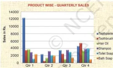
One more thing to remember: Excel redraws the chart automatically whenever the underlying data changes, so your formatting is never lost when you edit numbers — only the plotted values update.
Changing the Chart Type: When a Column Chart Can Become a Pie
A chart can be switched to another type at any time. The book demonstrates this by converting the quarterly column chart into a pie (NCERT, p. 113). Figure 4.9 shows the result. The conversion is safe because three conditions hold (NCERT, pp. 113-114):
- only one data series is plotted;
- all plotted values are positive;
- no plotted value equals zero.
Excel will not plot more than seven categories in a pie chart, because the categories represent the parts of the whole pie (NCERT, p. 114). If your data has more than seven parts, a pie is not the right chart.
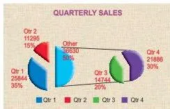
The book lists a 20-step procedure for creating the pie (NCERT, p. 114), but every step is a menu click. The grouped revision version:
- Enter the data, then select from two consecutive columns only — the labels column and the values column.
- Choose Pie from the Ribbon, then the 3-D Pie subtype.
- Use the Design tab to apply a chart layout and a chart style.
- Use the Format tab for shape effects such as bevel and shadow on the pie slices.
- Under Format Selection, set the angle of the first slice anywhere between 0 and 360 degrees to rotate the pie for a better view.
The takeaway: the 20 steps are just navigation. If you know which tab does what, you already know the whole procedure.
2-D and 3-D Charts: X, Y and the Depth Axis
In a 2-D chart, the horizontal X-axis holds categories (independent values) and the vertical Y-axis holds data (dependent values): the known value goes on X and the derived value on Y. The book’s example: to plot monthly demand in rupees, Month goes on the X-axis and the demand values on the Y-axis (NCERT, p. 115).
The intersection of the two axes is the origin (O). Positive values sit to the right of and above the origin; negative values sit to the left and below. So profit appears as positive data and loss as negative data (NCERT, p. 115).
Excel’s 2-D chart types are listed on page 116: line graphs, bar, area, surface column (horizontal or vertical), multiple line charts, radar chart, XY (scatter) and bubble chart.
A 3-D chart adds a third depth axis, also called the series axis or Z-axis, so data can be plotted along the depth of the chart (NCERT, p. 116). The book’s volume example needs three parameters: height on Y, length on X and breadth on Z. Figure 4.11(b) shows how a 3-D chart looks on screen.
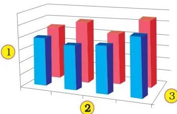
Use 3-D only when the third dimension carries real information, such as volume. If Z adds nothing meaningful, a 2-D chart stays clearer.
2-D vs 3-D at a glance
| Feature | 2-D chart | 3-D chart |
|---|---|---|
| Axes used | X (category) and Y (value) | X, Y plus Z (depth/series axis) |
| What each axis holds | X = independent values or categories; Y = dependent/derived values | Third axis plots data along the chart’s depth |
| Origin and negatives | Intersection of X and Y is the origin; positives right/up, negatives left/down | Same logic, extended along the depth |
| Types in the chapter | Line graphs, bar, area, surface column, multiple line, radar, XY (scatter), bubble | 3-D forms of charts, including the 3-D pie used in the chapter |
| When to choose it | Most business data; easy to read | When a third variable matters, e.g., volume (height, length, breadth) |
Two axis-absence rules complete the picture: radar charts have no horizontal (category) axis, and pie and doughnut charts have no axes at all (NCERT, p. 116).
Radar and Doughnut Charts: Special-Purpose Charts
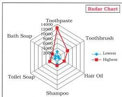
Data arranged in columns or rows on a worksheet can be plotted as a radar chart, which compares the aggregate values of several data series (NCERT, p. 116). The book builds one from the six products’ lowest and highest quarterly sales — each product pairs its lowest and highest figure, so the radar compares the spread across products.
Radar charts do not have a horizontal (category) axis.
The doughnut chart works on the same parts-to-a-whole idea as a pie, but it can contain more than one data series — each ring represents one series (NCERT, p. 117). Two subtypes exist: Doughnut (data in rings, one ring per series) and Exploded Doughnut (shows each value’s contribution to the total while emphasising individual values, again with more than one series).
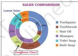
The book adds an honest caveat: doughnut charts are not easy to read, so a stacked column or stacked bar chart is often a better choice (NCERT, p. 117).
Why Use Charts at All? Explore, Present, Convince
The book gives charts three jobs (NCERT, p. 117):
- Help to explore — a chart shows possible relationships between variables immediately. The book’s examples are the relationship between a country’s GNP and its infant mortality rate, and between age and gender. Paging through raw data to find such links is slow; a chart shows them at a glance.
- Help to present — charts convey information in the least possible time. The book notes that newspapers and magazines such as The Economic Times and India Today were early users of charting techniques to sum up the ideas in their articles.
- Help to convince — graphs compress large amounts of information into exhibits that easily persuade an audience.
Tie this back to the chapter’s data thread: a quarterly sales chart instantly shows which product is growing and which is slipping — exactly the insight a manager needs before a business decision. That is the “useful in business decisions” point the chapter’s first question asks for.
Worked Example: Bar Chart and Pie Chart From a New Dataset
Method: two-step chart creation — enter data, then select and chart (NCERT, Section 4.1, p. 107). Company: Meera Electronics. Four products — LED Bulbs, Phone Chargers, Power Banks and USB Cables — with quarterly sales in rupees over four quarters (Qtr1 to Qtr4).
Step 1 — Enter data and compute totals. Put product names in rows and quarters in columns, with a Total column; then add a Total row for the quarters. The worksheet:
| Product | Qtr1 | Qtr2 | Qtr3 | Qtr4 | Total |
|---|---|---|---|---|---|
| LED Bulbs | 3200 | 4000 | 4800 | 4000 | 16000 |
| Phone Chargers | 2400 | 3000 | 3600 | 3000 | 12000 |
| Power Banks | 2000 | 2600 | 3200 | 4200 | 12000 |
| USB Cables | 2000 | 2400 | 2800 | 800 | 8000 |
| Total | 9600 | 12000 | 14400 | 12000 | 48000 |
Work one product total and one quarter total in full:
\[ 3200 + 4000 + 4800 + 4000 = 16000 \]
The LED Bulbs row totals Rs 16,000.
\[ 3200 + 2400 + 2000 + 2000 = 9600 \]
The Qtr1 column totals Rs 9,600. The remaining rows and columns follow the same pattern, giving quarter totals of Rs 9,600, 12,000, 14,400 and 12,000.
Grand total by the quarter route:
\[ 9600 + 12000 + 14400 + 12000 = 48000 \]
Grand total by the product route:
\[ 16000 + 12000 + 12000 + 8000 = 48000 \]
The two routes agree at Rs 48,000, so the entries are consistent.
Step 2 — Draw the product-wise bar chart. Select the Product column (labels) and the Total column. Keep this as a tidy two-column layout — labels next to values — the layout every chart in the chapter expects. Insert a 2-D bar chart. The result is one bar per product showing its yearly total in Rs. Step 3 — Draw the quarter-wise column chart.
Select the quarter names (labels) with the quarter totals and insert a column chart. The chart shows the four quarterly totals: Rs 9,600, 12,000, 14,400 and 12,000.
Step 4 — Convert the column chart to a pie. Check the three conditions for a safe conversion: one data series plotted (the quarter totals only) — yes; all values positive — yes; no value equals zero — yes. Use the Change Chart Type command, choose Pie and then the 3-D Pie subtype. Four categories sit comfortably inside Excel’s seven-category pie limit — yes.
Step 5 — Verify the percentages by hand. Check the Qtr3 slice:
\[ \text{Qtr3 \%} = \frac{14400}{48000} \times 100 = 0.3 \times 100 = 30\% \]
Excel’s data label on the Qtr3 slice should therefore read 30%. The complete set of slices:
| Quarter | Value (Rs) | Slice % |
|---|---|---|
| Qtr1 | 9600 | 20% |
| Qtr2 | 12000 | 25% |
| Qtr3 | 14400 | 30% |
| Qtr4 | 12000 | 25% |
Check the whole pie: 20 + 25 + 30 + 25 = 100%. If a percentage label does not match your hand calculation, the usual cause is a wrong selection — a label or value column that should not be in the chart got included. The same check works for any slice of any pie in this chapter.
Common Mistakes Students Make in Graphs and Charts
| Mistake | Correct rule | How to check your answer |
|---|---|---|
| Students select the whole data block, totals included, before making a pie | Select only two consecutive columns — labels plus one value column — because a pie plots a single series from one value column (NCERT, p. 114) | Count the legend entries: a pie must show exactly one series |
| Students call the plot area the chart area | The chart area is the entire chart with all elements; the plot area is only the region bounded by the axes (X and Y in 2-D; X, Y and Z in 3-D) | Open the Chart Elements box on the Format tab — the name shown there tells you which area is selected |
| Students think a pie can show several data series | A pie holds one series only; use a doughnut (one ring per series) or a stacked column/bar for several series | If you need more than one legend entry, a pie is the wrong chart |
| Students rebuild the chart after editing numbers | Excel redraws the chart automatically when the data or its range changes (NCERT, p. 121) | Edit one cell and watch the chart update by itself |
| Students put the dependent values on the X-axis | Categories (independent values) go on the X-axis; derived values go on the Y-axis (NCERT, p. 115) | Read the axis labels: months or product names on X, rupee values on Y |
| Students expect a pie from negative or zero figures | A pie needs positive non-zero values and at most seven categories (NCERT, p. 114) | Scan the source values before converting a chart to a pie |
| Students treat 3-D as decoration | 3-D adds a depth (Z) axis; use it when the third dimension carries information, such as volume (NCERT, p. 116) | Ask: if the Z-axis were removed, would the chart lose real meaning? If not, keep 2-D |
Exam Notes: How to Write Complete Answers
These skeletons map to the short-answer questions at the end of the chapter (NCERT, p. 122).
- Definition questions (define charts, graphs and their use in business decisions): open with the definition — a graph is a pictorial representation of data with at least a two-dimensional relationship — then name the two axes (X horizontal, Y vertical), then give the three advantages in order: explore, present, convince.
- Purpose questions (usage and purpose of column, pie and line charts): give one purpose plus one supporting point each. Column charts handle both comparisons among items and changes over a period of time; pie charts show the relative share of different elements of a whole; line charts show how a value changes over time.
- Description questions (data series, legend, data labels): define each term and connect them — related data points plotted together form a data series and appear as same-colour markers; the legend identifies each series in a chart; data labels add extra information about a data marker.
- Differentiation questions (pie vs line vs column; area vs XY chart vs doughnut; 2-D vs 3-D): answer as a small table — what each chart plots, how many axes or series it uses, and when to use it. Stay inside the chapter’s facts: doughnut shows parts-to-whole with more than one series and is hard to read; area and XY (scatter) are 2-D types; radar has no category axis; pie and doughnut have no axes at all.
- Step questions (move, resize and reposition a chart): numbered steps — click the chart to select it; for resizing, move the cursor to a corner or border until it becomes a two-headed arrow, then drag; for repositioning, drag the selected chart to the new location (NCERT, p. 115).
- Calculation questions (what a percentage in a chart represents and how the software calculates it): each slice’s value divided by the total, times 100; the whole pie equals 100% (NCERT, p. 113).
- Broad questions (types of charts Excel can prepare): enumerate the 2-D list — line graphs, bar, area, surface column (horizontal or vertical), multiple line charts, radar chart, XY (scatter) and bubble chart — then add pie, doughnut and the 3-D forms (NCERT, p. 116).
- The how-to-prepare question (describe the use of Excel for preparation of a chart): the eight-step routine on page 119 is the complete answer — enter data; create a basic chart; change layout or style; add or remove titles and data labels; show or hide the legend; display or hide axes and gridlines; move and resize the chart; save the chart.
Skill Review Decoded: What Each Practice Task Teaches
The chapter’s practice tasks A to G (NCERT, p. 123) look repetitive, but each one drills a different chart skill. The decoder:
| Task | Data to enter | Chart to build | Skill it trains |
|---|---|---|---|
| A | Population literate and illiterate data for males and females, years 2001-2008 | Trend chart | Line charts for time-series data |
| B | The Total column (column 3) of that table | Pie chart | Showing parts of a whole |
| C | Separate tables for male, female and total | Trend charts for each | Multiple line charts comparing series over time |
| D | Literate and illiterate figures for each gender | Column charts | Comparing absolute values |
| E | Ten plot areas: 5, 7, 8, 9, 8, 10, 4, 6, 7 and 3 hectares | Pie chart and column chart | Seeing the same data two ways — all values are positive, but ten categories exceed the seven-category pie limit |
| F | RTO vehicle registrations: bus, trucks, auto rickshaw, cars, two wheelers and heavy vehicles | Pie chart | Six categories stay inside Excel’s seven-category pie limit |
| G | Marks distribution of 1000 students from 0-20 up to 81-100 | Column chart | Grouped categories compared side by side |
Takeaway line: line = trend, pie = share, column = compare.
Quick Revision: The Chapter in One Page
| Chart type | Purpose | Constraint to remember |
|---|---|---|
| Line (single or multi) | Trend of a value over time | Categories on the X-axis |
| Column | Comparisons among items and changes over a period of time | Versatile default for business data |
| Bar | Comparison of absolute values at discrete points (time intervals, products) | Depicts two or more variables |
| Pie | Share of a whole | One series; at most seven categories; positive non-zero values only |
| Doughnut | Parts-to-whole with several series | Not easy to read — a stacked column or bar is often better |
| Radar | Compare aggregate values of several data series | No horizontal (category) axis |
The chapter’s eight-step routine for preparing any chart (NCERT, p. 119):
- Enter data in a worksheet with proper column and row titles.
- Create a basic chart using a pattern from the Chart group’s panel at the top of the worksheet.
- Change the layout or style — apply a predefined chart layout, apply a predefined chart style, change the layout of chart elements, change the format of chart elements.
- Add or remove titles and data labels — chart title, axis titles, a title linked to a worksheet cell, data labels.
- Show or hide the legend.
- Display or hide chart axes or gridlines — primary axes, secondary axes, gridlines.
- Move or resize the chart.
- Save the chart.
Memory device — the axes: “X sits, Y stands, Z goes back.” X is the horizontal category axis, Y is the vertical value axis, and Z is the depth axis of a 3-D chart. In three words: X categories, Y values, Z depth.
Memory device — the chart elements: the sentence “Can’t Plot Data – Ask Legend To Draw” preserves the element order: Chart area, Plot area, Data (points, markers and series), Axes, Legend, Titles, Data labels.
Final checklist for the night-before scan: chart area, plot area, data, axes, legend, titles and data labels — if all seven are covered, the chapter is revised. For the rest of your revision, browse the Class 12 notes hub or the complete CBSE notes index.
Frequently Asked Questions
Why can Excel pie charts show only seven categories?
Excel cannot plot more than seven categories in a pie chart, and the categories represent the parts of the whole pie (NCERT, p. 114). If your data has more than seven parts, choose a different chart such as a column chart or a doughnut chart instead.
What is the difference between chart area and plot area?
The chart area is the entire chart, including all its elements — title, legend, labels and everything else. The plot area is only the region in which the data is plotted: bounded by the X and Y axes in a 2-D chart, and by the X, Y and Z axes in a 3-D chart (NCERT, pp. 108-109).
Does Excel redraw a chart automatically when the data changes?
Yes. Excel automatically redraws the chart if any change is made in the data or in the range of data (NCERT, p. 121). You do not need to rebuild a chart after editing a value.
How does Excel calculate the percentage shown in a pie chart?
Excel divides the slice’s value by the total of all plotted values and multiplies by 100, and the whole pie always equals 100% (NCERT, p. 113).
\[ \text{Slice \%} = \frac{\text{slice value}}{\text{grand total}} \times 100 \]
In the worked example above, the Qtr3 slice is (14400 / 48000) × 100 = 30%.
Which chart should I use to compare quarterly sales of products?
A column chart (or bar chart) is the natural choice — column charts handle both comparisons among items and changes over a period of time (NCERT, p. 120).
If you want each product’s or quarter’s share of the year’s total instead, convert to a pie: select the labels plus their totals in two consecutive columns, and keep the categories at seven or fewer.
What is the difference between a 2-D and a 3-D chart?
A 2-D chart plots data on two axes: the horizontal category axis (X) for independent values and the vertical value axis (Y) for dependent values. A 3-D chart adds a third depth axis (Z), also called the series axis, so data can be plotted along the depth of the chart (NCERT, p. 116).
Use 3-D only when the third dimension carries real information — like volume, which needs height (Y), length (X) and breadth (Z).
Reference: NCERT Class 12 Accountancy textbook, chapter 4, Graphs and Charts.
Explore Class 12 Accountancy Notes
- Class 12 Accountancy Notes
- Class 12 CBSE Notes
- CBSE Notes for Classes 1 to 12
- Previous: Spreadsheet
Class 12 Accountancy on LearnCBSE:
Related chapters:
- Overview of Computerised Accounting System notes
Official source: download the NCERT textbook free from ncert.nic.in.