
These Spreadsheet Class 12 notes revise Chapter 2 of the NCERT Class 12 Accountancy book, Computerised Accounting System, for the 2026-27 session (Rationalised NCERT). A spreadsheet is a configuration of rows and columns — also called a worksheet — used to record, calculate and compare numerical or financial data.
Every value in it is either basic (typed independently) or derived (computed from other values through an arithmetic expression or a function).
One edition note matters before revision: the chapter teaches MS-Excel 2007 with 65,536 rows, 256 columns, the Ribbon interface and the Office Button. Later Excel versions provide more than a million rows and use a File tab instead of the Office Button, but every concept here — cell references, formulas, functions, named ranges, what-if analysis — works the same way in current versions.
The grounded scope of these notes runs from page 17 to page 50 of the chapter.
What a Spreadsheet Is, and the Chapter Roadmap
A spreadsheet is recorded, calculated and compared data arranged as rows (horizontal vectors) and columns (vertical vectors). A spreadsheet application is the computer program that lets you enter and process that data; the book explains everything through MS-Excel, a member of the Microsoft Office Suite (NCERT, p. 17).
Excel 2007 uses a redesigned interface built around a series of horizontal tabs called the Ribbon. The Office Button (upper-left corner) handles opening an old workbook, creating a new one, saving, and printing — jobs the old File menu used to do (NCERT, p. 17-18).
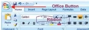
Figure 2.1 shows the Excel 2007 window: the Ribbon of horizontal tabs across the top organises commands, and the Office Button in the upper-left opens, creates, saves and prints workbooks. The chapter then teaches a small number of building blocks that this page follows in the same order:
- Worksheet basics — workbook, sheets, active worksheet
- Cells and references — row/column addresses, relative, absolute and mixed references
- Values and labels — basic versus derived values, auto-detected data types
- Formulas — the mandatory
=sign and the order of operations - Functions — SUM, AVERAGE, COUNT and the twelve-category function library
- Named ranges and IF / nested IF — readability and conditional logic
- Function groups — date, mathematical, text, logical, lookup and financial
- Data entry, fill options and importing text data
If you are revising the whole book, read the overview of the computerised accounting system first (Chapter 1), then this chapter, then graphs and charts (Chapter 3). Browse all subjects from our CBSE notes index, or jump straight to the Class 12 notes and the Class 12 Accountancy notes hub.
Workbook, Worksheets and the Active Sheet
Understand the file structure first: a workbook is simply an Excel file, and it holds a collection of worksheets (NCERT, p. 18). By default, three sheets — Sheet 1, Sheet 2, Sheet 3 — are available. Only one worksheet can be active at a time, and the active worksheet is the one you can operate on.
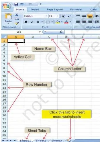
Figure 2.2 shows the sheet tabs at the bottom of the workbook window. The name of the active worksheet appears in bold on its Sheet Tab at the bottom left.
- Add a sheet: click the Insert Worksheet icon next to the tabs.
- Rename a sheet: right-click the sheet name, then choose Rename.
Cells, Cell Addresses, Ranges and Navigation
In Excel 2007, rows are numbered 1 to 65,536 from top to bottom, and columns are lettered A to IV from left to right — 256 columns in all. That gives roughly 1,65,00,000 cells per sheet, the book’s own approximation (NCERT, p. 19).
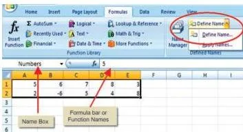
Figure 2.3 shows the grid: row numbers run down the left, column letters across the top. A cell is the intersection of a row and a column — the first cell, A1, sits at row 1 under column A. Each cell has a unique cell address (a letter plus a number, such as G8).
When Excel starts, the cursor points at A1; that cell is the active cell (NCERT, p. 19).
A range is a group of cells named by its upper-left and lower-right corners separated by a colon — A1:E2 tells Excel to include every cell between A1 and E2. Cell references are used in formulas, functions, charts and other Excel commands (NCERT, p. 19).
The three reference types, and what copying does to each
Think of a relative reference as directions — “two cells above me” — and an absolute reference as a fixed landmark that never moves. The default is relative: copy a formula and its references adjust to the new location. Lock a cell with dollar signs ($C$4) to keep it fixed.
A mixed reference locks only one part: $C4 fixes the column, C$4 fixes the row (NCERT, p. 19).
| Reference type | Example | After copying one cell down | Use it when |
|---|---|---|---|
| Relative | C4 | becomes C5 | the same formula must repeat down a column (the default) |
| Absolute | $C$4 | stays $C$4 | one fixed input, like a rate or tax cell, must never move |
| Mixed | C$4 | stays C$4 (row locked) | keep the row constant while the column changes |
| Mixed | $C4 | becomes $C5 (column locked) | keep the column constant while the row changes |
Navigating the worksheet with keystrokes
The mouse handles almost everything except data entry, but these key strokes move the cursor faster (NCERT, p. 20):
| Movement | Keystroke |
|---|---|
| One cell down | Down arrow or Enter |
| One cell up | Up arrow |
| One cell left | Left arrow |
| One cell right | Right arrow or Tab |
| Top of worksheet (cell A1) | CTRL + HOME |
| Last row/last column containing data | CTRL + END |
| Skip between filled clusters in a row | CTRL + Right arrow or END + Right arrow |
| Skip between filled clusters in a column | CTRL + Down arrow or END + Down arrow |
| Beginning of the current row | HOME |
Values, Labels and the What-If Idea
The chapter’s first idea is the difference between a basic and a derived value (Box 2.1, NCERT p. 18). If quantity Q of an item is bought at price P, then \[ V = Q \times P \]
P and Q are basic values (entered directly); V is the derived value because it is obtained by multiplying Q with P; and Q × P is called an arithmetic expression. An arithmetic expression may itself contain one or more functions (NCERT, p. 18).
Excel also auto-detects what you type. Enter 306 and it is taken as numeric; enter Asset and it is alpha-numeric; enter 12/07/08 and it is treated as a date (NCERT, p. 20-21).
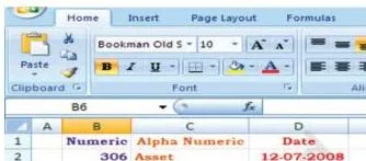
Figure 2.5 illustrates exactly that: the same worksheet shows a number, a text word and a date, each recognised by its own nature. Labels (NCERT, p. 22) are the text or descriptive entries — anything beginning with A-Z, such as Principal Amount or Maturity Amount — and they cannot be used in arithmetic: labels cannot be multiplied or subtracted.
The value rule, credited to computer scientist Alan Kay (NCERT, p. 21), states that a cell’s value relies solely on the formula the user typed into that cell. That formula may depend on other cells, but those are likewise restricted to entered data or formulas.
There are no side effects: the only output is the calculated result displayed in the cell, and nothing else is modified unless you change it manually.
A what-if scenario is what this rule makes possible: change one or more input (basic) values and all derived values revise themselves automatically, so you can examine the cause (if) and effect (what) of variations in inputs (NCERT, p. 22). Think of a spreadsheet as a calculator with visible wiring: touch any input and every connected output recalculates instantly.
The chapter’s planning step matters before you type anything: decide which cells will hold values and which cells will hold the relationships (formulas), and only then enter the data (NCERT, p. 21).
Reading Figure 2.6: The Compound Interest Worksheet Layout
The book’s running example — compound interest and maturity amount on a fixed deposit — is the best demonstration of that planning step. Six cells are defined with column headings (NCERT, p. 21):
- Principal Amount (PA) — column B
- Rate of Interest (r) — column C
- Period of Compounding (CP) — column D
- Period in years (NY)
- Maturity Amount (MA) — column E
- Compound Interest (CI) — column F
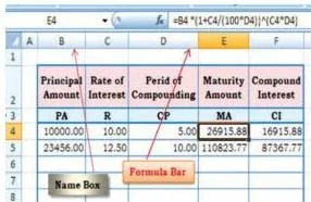
Figure 2.6 shows the finished fixed-deposit layout for yearly compounding. The basic values are typed directly into B4 (principal), C4 (rate) and D4 (compounding periods). The derived values MA and CI are computed by formulas in E4 and F4, and when you select a derived cell, its formula is visible in the formula bar.
Change any basic value (say, the rate in C4) and E4 and F4 revise automatically — that automatic recalculation is the mechanism behind every what-if scenario.
The chapter’s formulas, in the book’s notation, are (NCERT, p. 21-22):
\[ MA = PA \times \left(1 + \frac{R}{100 \times CP}\right)^{R \times CP} \]
\[ CI = MA – PA \]
Symbol meanings: PA = principal amount in rupees, R = annual rate of interest in percent, CP = compounding periods per year, MA = maturity amount, CI = compound interest. The planning lesson: define cell headings first, enter basic data, then enter the relationships — the order is the method.
Formulas and the Order of Mathematical Operations
A formula is a mathematical calculation on a set of cells, and it must start with an = sign (NCERT, p. 22). In the book’s example the cell E3 holds =D1+E1/F1*G1 and displays the value 16.
A formula cell has two display components: when you click the cell, the formula bar shows the formula itself; at all other times the cell shows the resulting value (NCERT, p. 22-23).
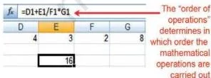
Figure 2.7 shows the two components side by side: the formula bar carries =D1+E1/F1*G1 while the cell displays the computed 16. A spreadsheet without any formulas is only a row-and-column list of data, like a calendar or timetable (NCERT, p. 23).
Excel follows the rules of algebra for the order of operations (NCERT, p. 23):
- Operations inside brackets are carried out first.
- Exponents come next.
- Division and multiplication are equal in importance and run left to right.
- Addition and subtraction are equal and also run left to right.
Why the order matters: in 2+3*4, multiplication runs first, so the result is 14 — not 20. The three mnemonics the book lists (GEMS, PEMDAS, BEMDAS) all describe the same five-step order:
| Step | GEMS | PEMDAS | BEMDAS | What it means |
|---|---|---|---|---|
| 1 | G = Grouping ( ) | P = Please — parenthesis ( ) | B = Brackets ( ) | evaluate inside brackets first |
| 2 | E = Exponents ^ | E = Excuse — exponents ^ | E = Exponents ^ | powers before other operations |
| 3-4 | M = Multiplication * / Division | M = My (*), D = Dear (/) | M = Multiplication, D = Division | × and ÷ left to right |
| 5-6 | S = Subtraction / Addition | A = Aunt (+), S = Sally (−) | A = Addition, S = Subtraction | + and − left to right |
The Formula tab of the ribbon contains four sections: functions library, defined names, formula auditing and calculation (NCERT, p. 23). Functions live in the first of these, covered next.
Functions: Excel’s Built-In Formulas
A function is a special key word you enter into a cell to process the data written inside its brackets — in effect a built-in set of formulas, entered as =FunctionName(Data) (NCERT, p. 23-24). Every function involves four issues you should be able to state for any function you use:
- Name of the function
- Purpose of the function
- The arguments (data) it needs to do its job
- The result it returns
SUM, AVERAGE and COUNT are the easiest functions. Each applies to a range of cells containing numbers (blank cells are allowed but text is not) and returns, respectively, the arithmetic total, the average (mean) value, or the quantity of values in the range (NCERT, p. 24). The AutoSum (Σ) button automates summation.
In the book’s example, clicking AutoSum at G5 and typing the range D1:G1 puts the answer 17 in G5 — the formula bar then shows =SUM(D1:G1) (NCERT, p. 24).
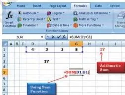
Figure 2.9(b) shows that AutoSum result: the range D1:G1 is marked, the total 17 appears in G5, and =SUM(D1:G1) is visible in the formula bar. AutoSum also offers AVERAGE, MIN, MAX and COUNT.
Excel 2007 provides twelve categories of functions on the ribbon (NCERT, p. 25). The book flags six of them as useful in computerised accountancy:
| Category | What it does | Functions taught in this chapter | NCERT page |
|---|---|---|---|
| Financial | money, loan and investment calculations | ACCRINT, CUMIPMT, PV, FV, PMT, RATE, NPV | p. 41-47 |
| Date and Time | date-time serial numbers and their parts | TODAY, NOW, DAY, MONTH, YEAR, DATEVALUE | p. 30-31 |
| Lookup and References | find values inside tables | LOOKUP, VLOOKUP, HLOOKUP | p. 36-41 |
| Database | work on lists as databases | listed as useful, but not detailed in the pages covered here | p. 25 |
| Text | manipulate text strings | TEXT, CONCATENATE | p. 34-35 |
| Logical | true/false decisions | IF, AND, OR | p. 27-29, 35-36 |
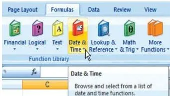
Figure 2.13 shows the categorised function library on the Formula tab, where the twelve categories appear grouped on the ribbon. Each family is examined in its own section below.
Named Ranges: Working with Names Instead of Cell Addresses
A named range replaces a cell range with a descriptive name, which saves time when writing complex formulas and makes them readable: =SUM(Numbers) is easier to remember than =SUM(B1:F1) (NCERT, p. 25). Behind the name, Excel still hides the cell references.
The steps for defining a name (NCERT, p. 25-26):
- Select the cells to be named (for example B1:F1).
- Click the Formula tab on the ribbon.
- Select Define Name and click it.
- In the New Name dialog, type the name (say, Numbers) in the Name window; the Refers to window shows $B$1:$F$1.
- Click OK; the name now appears in the Name Box.
- To use it, click Apply Names and choose the range name.
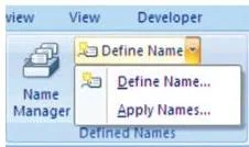
Figure 2.10(d) shows that New Name dialog: the Name window holds the descriptive name and the Refers to window shows the absolute address $B$1:$F$1. The grounded results to remember from the book’s sequence:
- =SUM(Numbers) in D3 totals the named range B1:F1 (NCERT, p. 26).
- =SUMIF(Numbers, “<6”) adds only the numbers less than 6 in that range and returns 9 (NCERT, p. 26).
- With two named ranges, =SUM(Monthly_Totals) (cells B2:B5) returns 1158 and =SUM(Monthly_Tax) (cells C2:C5) returns 238 (NCERT, p. 26-27).
- The balance cell B7 holds =Total_of_Month – Total_of_Tax, where those two names refer to B6 and C6 (NCERT, p. 27).
To stop recalculation and keep the present calculated values, freeze the formulas: select the formula cells (B6:C6, B7), go to Home → Copy → Paste Special, choose the Values radio button and click OK. This permanently removes the formulas and keeps only the current results (NCERT, p. 27) — the standard way to save a snapshot that must not change.
IF and Nested IF: Building Conditions into Cells
The IF function returns one value if a specified condition evaluates to TRUE and a different value if it evaluates to FALSE. Its format (NCERT, p. 27-28):
=IF(logical_test, value_if_true, value_if_false)
- logical_test — the value or expression judged true or false; it requires a logical operator ( =, <, <=, <>, >, >= ). There is no middle result: something is either true or false.
- value_if_true — returned when the test is true; can be a value, text, expression, formula, or a reference to another cell.
- value_if_false — returned when the test is false; same possibilities.
Book examples to recognise instantly: =IF(A1<20,”Yes”,”No”) returns Yes when A1 is below 20; =IF(C2>B2,(C2+D2)/2,(B2+D2)/2) returns (C2+D2)/2 if C2>B2, otherwise (B2+D2)/2 (NCERT, p. 28). The book’s saving-percentage table decides a value column: when the total crosses ₹10,000 the entry shows 10%, otherwise 5%, written as =IF(E4>10000, 10%, 5%) (NCERT, p. 28).
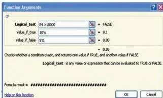
Figure 2.12(b) shows the Function Arguments dialog that walks a user through IF: type the condition in logical_test, the true-branch value, then the false-branch value, and click OK. This dialog is how the ribbon builds IF expressions step by step.
Nested IF for several conditions
When one condition is not enough, put an IF inside another IF: =IF(logical_test, IF(logical_test, IF(…), value_if_false), value_if_false) (NCERT, p. 29).
The book’s marks example, where E2 holds the marks and F2 the result, is =IF(E2<96, IF(E2<91, IF(E2<55,”Fail”,”C Grade”), “B Grade”), “A Grade”) Trace it: below 55 → Fail; 55-90 → C Grade; 91-95 → B Grade; 96 or more → A Grade.
The critical rule about nesting: if a nested function is used as an argument, it must return the same type of value that the argument uses. If the argument expects a TRUE/FALSE result and the nested function returns something else, Excel displays the #VALUE! error in the cell (NCERT, p. 29).
Date, Mathematical and Text Functions
Date and time functions
Excel stores dates as serial numbers so they can be calculated. By default, January 1, 1900 is serial number 1; January 1, 2009 is 39814 because it is 39,814 days later (NCERT, p. 30).
- TODAY() — returns the serial number of the current date.
- NOW() — like TODAY but includes the current time (times are fractions of a day).
- DAY(serial_number) — the day of the date, an integer 1 to 31 (a date of 16-Apr-2009 gives 16).
- MONTH(serial_number) — the month, 1 (January) to 12 (December).
- YEAR(serial_number) — the year, 1900 to 9999.
- DATEVALUE(date_text) — converts a date written as text into a serial number; =DATEVALUE(“16-04-2009”) returns 39919 (NCERT, p. 30).
The book’s age example divides the difference of two dates by 365.25 — the fraction allows for leap years — to convert days into years (NCERT, p. 31).
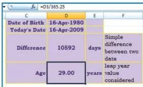
Figure 2.17 shows that age layout: the date difference sits in D3, and dividing it by 365.25 expresses the age in years, leap years included.
Mathematical functions
SUMIF(range, criteria, sum_range) adds only the cells that satisfy a criterion. The criteria can be a number, an expression or text — for example 1500, “>1500” or “Books” (NCERT, p. 31).
The book’s grounded depreciation example: asset values are in D2:D5 and their depreciation in E2:E5, and =SUMIF(D2:E5, “>150000”, E2:E5) adds the depreciation of asset values above ₹1,50,000 and returns ₹63,000 (NCERT, p. 31).
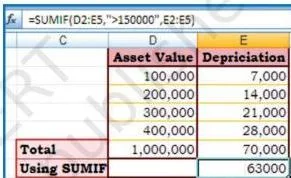
Figure 2.18 shows the depreciation worksheet behind that formula: the range D2:D5 holds asset values, E2:E5 the related depreciation, and the SUMIF result 63,000 appears in E7.
ROUND(number, num_digits) rounds a number to a specified number of digits (NCERT, p. 31). The three cases for num_digits:
- Greater than 0 — round to that many decimal places: =ROUND(3.14159, 2) gives 3.14.
- Equal to 0 — round to the nearest integer: =ROUND(21.5, 0) gives 22.
- Less than 0 — round to the left of the decimal point: =ROUND(147, -2) gives 100.
ROUNDUP rounds away from zero (3.2 → 4 at 0 digits) while ROUNDDOWN rounds toward zero (3.2 → 3), and both accept negative num_digits the same way ROUND does (NCERT, p. 32).
The COUNT family decides what counts (NCERT, p. 32-33):
- COUNT counts only cells containing numbers — dates count as numbers; text, blank cells, logical values and error values are ignored.
- COUNTA counts every non-blank entry, including text, logical values and errors.
- COUNTBLANK counts only the empty cells.
- COUNTIF(range, criteria) counts cells in a range that meet one criterion, written as 32, “>32”, “apples” or a cell reference (NCERT, p. 33-34).
Two dimension functions support array work: ROWS(array) returns the number of rows and COLUMNS(array) the number of columns in a reference or array. An array is a group of arguments arranged in rows and columns; an array formula performs multiple calculations and is enclosed in braces { } and entered by pressing CTRL+SHIFT+ENTER (NCERT, p. 33).
Text functions
TEXT(value, format_text) converts a numeric value to text in a specific number format (NCERT, p. 34). If cell L1 holds 23.5, then =TEXT(L1, “Rs 0.00”) displays Rs 23.50. CONCATENATE(text1, text2, …) joins 2 to 255 text items into one text string — the book’s example builds each employee’s Full Name from First Name, Middle Name and Last Name cells (NCERT, p. 34-35).
Logical and Lookup Functions: AND, OR, LOOKUP, VLOOKUP, HLOOKUP
AND and OR
AND returns TRUE only if every argument is TRUE; OR returns TRUE if any argument is TRUE. Both accept up to 255 logical values (NCERT, p. 35-36). The classic exam-style combination wraps AND inside IF as the logical test:
=IF(AND(A2>1, A2<100), A2, “The value is out of range.”) With A2 holding 50, the function returns 50; for a value outside 1-100 it returns the message (NCERT, p. 35).
LOOKUP: vector and array forms
The vector form, LOOKUP(lookup_value, lookup_vector, result_vector), searches a one-row or one-column range and returns a value from the same position in a second range (NCERT, p. 36). Two rules decide its results:
- The lookup_vector must be in ascending order (-2, -1, 0, 1, 2 or A-Z), otherwise LOOKUP may return a wrong value (NCERT, p. 37).
- If no exact match exists, LOOKUP matches the largest value less than or equal to the lookup value; if the lookup value is smaller than the smallest vector value, it returns #N/A (NCERT, p. 37).
The book’s colour-frequency table (NCERT, p. 37) shows this: =LOOKUP(4.19, A2:A6, B2:B6) returns orange; =LOOKUP(5.00, …) also returns orange (the largest value ≤ 5.00 is 4.19); =LOOKUP(0, …) returns #N/A.
The array form, LOOKUP(lookup_value, array), searches the first row or first column of the array depending on its shape — if the array is wider than tall it searches the first row, otherwise the first column (NCERT, p. 37-38).
VLOOKUP and HLOOKUP
VLOOKUP (vertical lookup) searches the first column of a table and returns a value from any cell on the same row (NCERT, p. 38).
=VLOOKUP(lookup_value, table_array, col_index_num, range_lookup)
- lookup_value — the value searched in the first column; if it is smaller than the smallest first-column value, VLOOKUP returns #N/A.
- table_array — two or more columns of data; use a range reference or a range name.
- col_index_num — the column of the table to return from (1 = first column, 2 = second, and so on). Less than 1 gives #VALUE!; greater than the number of columns gives #REF! (NCERT, p. 38-39).
- range_lookup — FALSE demands an exact match (the first column need not be sorted; if two values match, the first found is used). TRUE or omitted permits an approximate match, but then the first column must be sorted ascending or results go quietly wrong (NCERT, p. 39).
The employee example (NCERT, p. 39) uses =VLOOKUP(A3, A1:D7, 4, FALSE): for employee code 3456 in A3, the fourth column (Basic Pay) returns 3,453.00.
HLOOKUP (horizontal lookup) is the twin that searches the first row of a table and returns a value from the same column in another row (NCERT, p. 40). Its syntax is =HLOOKUP(lookup_value, table_array, row_index_num, range_lookup). The book’s budget example pulls each quarter’s budget from Worksheet 1 into Worksheet 2:
=HLOOKUP(C4, Budget!$A$1:$E$2, 2, FALSE) Read it: C4 is the quarter, Budget! is the sheet holding the table, $A$1:$E$2 is the absolute table array, 2 is the row to return, and FALSE asks for an exact match (NCERT, p. 40-41).
The chapter’s caution applies to all lookup functions: table arrays should be converted to absolute cell references so the range does not shift when formulas are copied (NCERT, p. 41).
Financial Functions for Accountancy
Business input frequently contains dates, interest rates and tax percentages, while output needs age, depreciation, future value and net present value — exactly what the financial library provides (NCERT, p. 29). Two cross-cutting rules govern all of them:
- Match units: rate and nper must use the same time unit. A monthly payment plan over 48 months needs the monthly rate 10%/12 with nper = 48 (NCERT, p. 43).
- Sign encodes direction: money you pay out is entered negative, money you receive positive. The book’s car-loan example enters pmt = -263.33 for a monthly payment (NCERT, p. 43).
Excel solves one financial argument in terms of the others through this underlying equation (NCERT, p. 43):
\[ pv \times (1 + rate)^{nper} + pmt \times (1 + rate \times type) \times \frac{(1 + rate)^{nper} – 1}{rate} + fv = 0 \]
When rate is 0, the same equation reduces to pmt × nper + pv + fv = 0 (NCERT, p. 43). This is why a negative pmt balances a positive pv — signs are the equation’s built-in direction code.
Function-by-function reference
| Function | Syntax | Use in accountancy | Sign / unit notes | Page |
|---|---|---|---|---|
| ACCRINT | (issue, first_interest, settlement, rate, par, frequency, basis, calc_method) | accrued interest for a security that pays periodic interest | frequency 1/2/4 = annual/semi-annual/quarterly; par defaults to 1000; enter dates with DATE() | p. 41-42 |
| CUMIPMT | (rate, nper, pv, start_period, end_period, type) | cumulative interest paid between two periods of a loan | type 0 = end of period, 1 = beginning; results are negative (interest paid out) | p. 42 |
| PV | (rate, nper, pmt, fv, type) | present value of a stream of future payments — a loan amount is the PV | rate and nper in the same unit; pmt negative when paying out | p. 42-43 |
| FV | (rate, nper, pmt, pv, type) | future value of regular savings with compound interest | type changes the result: book’s ₹200 monthly example gives ₹2,581.40 (type 1) vs ₹2,571.18 (type 0) | p. 44 |
| PMT | (rate, nper, pv, [fv], [type]) | periodic payment for a fixed-rate loan or mortgage | the payment comes back negative because it flows out | p. 45 |
| RATE | (nper, pmt, pv, fv, type, guess) | interest rate per period implied by the other terms | found by iteration; guess defaults to 10%; returns #NUM! if it does not converge in 20 iterations | p. 45-46 |
| NPV | (rate, value1, value2, …) | net present value of an investment with unequal cash flows | 1-254 values, equally spaced at the end of each period; order matters | p. 46 |
The formula behind ACCRINT, as the book prints it, is (NCERT, p. 42):
\[ ACCRINT = par \times \frac{rate}{frequency} \times \sum \frac{A’}{NL} \]
And NPV is built from the discounted sum of the cash flows (NCERT, p. 46):
\[ NPV = \sum_{i=1}^{n} \frac{values_i}{(1 + rate)^i} \]
Which function to reach for
| Function | The accounting question it answers | Behaviour to remember |
|---|---|---|
| PV | What is a future stream of payments worth today (for example, the loan amount)? | cash flows must be constant; type places them at end or beginning of period (p. 42-43) |
| FV | What will regular savings grow to in the future? | type shifts the result significantly, as the ₹2,581.40 vs ₹2,571.18 book pairs show (p. 44) |
| PMT | What fixed payment repays this loan? | the answer is negative — it is money you pay out (p. 45) |
| RATE | What interest rate do these terms imply? | computed by iteration; fails to #NUM! if it cannot converge (p. 45-46) |
| CUMIPMT | How much interest is paid between two specific periods? | needs start_period and end_period; type 0 or 1 for timing (p. 42) |
| NPV | Is this investment worth its cost at a given discount rate? | allows unequal cash flows; IRR is the rate at which NPV = 0 (p. 46) |
Also note the PV-versus-NPV distinction the book draws: PV requires constant cash flows through the investment, while NPV accepts variable cash flows, which is why NPV is the tool for uneven project returns (NCERT, p. 46).
Data Entry, Fill Options and Importing Text Data
Input data — payroll parameters such as month name, working days or DA% — must be correct, accurate and in proper format before the software processes it (NCERT, p. 47). Two defaults to memorise:
- Numbers are right-aligned in a cell by default.
- Text is left-aligned by default.
Excel also recognises a date, currency or percentage value on entry. Type 16/04/1980 and the spreadsheet treats it as a date and acts accordingly (NCERT, p. 47).
Filling a series with the fill handle
The fill handle is the small black square in the lower-right corner of a selection; when you point at it, the pointer becomes a black cross. Dragging it fills adjacent cells with a continued series (NCERT, p. 47-48). The book’s example: if A1 holds 10 and A2 holds 20, dragging the fill handle from A2 down to A10 produces 10, 20, 30, … 100 in steps of 10.
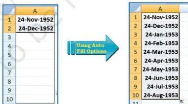
Figures 2.34 and 2.35 show that drag method: 10 and 20 are already entered, and dragging the handle continues the series to 100. The same effect is available through Home → Fill → Series, where Step Value 10 and Stop Value 100 fill the range automatically (NCERT, p. 48-49). Date series fill the same way once the cells are formatted as dates via Format Cells.
Importing data from a text file
Data can also be copied or imported from text files, which a text editor such as Notepad reads directly. Such files often carry the extension .txt or .csv — Comma Separated Values (NCERT, p. 49). The outline of the import route:
- Create the data file in Notepad: one line = one row; entries separated by commas = columns; the first line can hold the column names.
- Open a new Excel worksheet from the Office Button.
- Select the Data tab on the ribbon.
- Choose Get External Data → From Text and select the Notepad file.
- Excel places each comma-separated value into its own column and row (NCERT, p. 49-50).
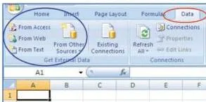
Figure 2.40 shows the From Text step of that process — the dialog that locates the .csv file and converts it into worksheet rows and columns. This import idea leads to the chapter’s final classification: a cell holds four kinds of data (NCERT, p. 50):
- Labels (text) — descriptive data such as names and months; left-aligned.
- Values (numbers) — whole or decimal values, right-aligned. A trailing zero note: entering 246.70 displays as 246.7 unless you change the display format.
- Formulas — instructions for Excel to perform calculations.
- Dates — entering 16/12 displays as 16-Dec while the formula bar shows 16/12/2008 (the exact format depends on the country-specific format setting).
Spreadsheet Definitions at a Glance
Revise every key term from one table. Meanings are given in student-friendly wording, each with a concrete example and the chapter page for lookup.
| Term | Meaning | Example | Page |
|---|---|---|---|
| Spreadsheet / worksheet | a configuration of rows and columns used to record, calculate and compare numerical or financial data | an Excel sheet set out in rows and columns | p. 17 |
| Workbook | an Excel file; a collection of worksheets | one Excel file with Sheet 1, Sheet 2, Sheet 3 | p. 18 |
| Active worksheet | the single worksheet available for operations at one time | its name appears in bold on the Sheet Tab | p. 18 |
| Row | a horizontal vector of cells, numbered from top to bottom | rows 1 to 65,536 in Excel 2007 | p. 19 |
| Column | a vertical vector of cells, lettered left to right | columns A to IV (256 columns) in Excel 2007 | p. 19 |
| Cell | the intersection of a row and a column, where a value, function or expression is recorded | the box at row 1, column A | p. 19 |
| Cell address | the unique letter-plus-number identification of a cell | A1, G8 | p. 19 |
| Active cell | the cell currently pointed to by the cursor | A1 when Excel starts | p. 19 |
| Range | a group of cells named by upper-left and lower-right corners separated by a colon | A1:E2 includes all cells between A1 and E2 | p. 19 |
| Relative reference | the default reference; adjusts when a formula is copied to a new location | copying =C4 one cell down makes it =C5 | p. 19 |
| Absolute reference | a reference fixed with dollar signs so it never changes on copy | $C$4 | p. 19 |
| Mixed reference | a reference holding either the row or the column constant | $C4 (column fixed) or C$4 (row fixed) | p. 19 |
| Basic value | a value entered directly, not calculated | price P or quantity Q in V = Q × P | p. 18 |
| Derived value | a value computed from other values by an expression or function | V in V = Q × P | p. 18 |
| Arithmetic expression | a calculation on values; may contain functions | Q × P | p. 18 |
| Label | descriptive text beginning with A-Z; cannot be used mathematically | Principal Amount | p. 22 |
| Formula | a mathematical calculation on a set of cells, always starting with = | =D1+E1/F1*G1 | p. 22 |
| Formula bar | the display that shows a cell’s formula when that cell is selected | selecting E3 shows =D1+E1/F1*G1 | p. 22 |
| Function | a built-in set of formulas entered as =FunctionName(Data) | =SUM(D1:G1) | p. 23-24 |
| Argument | the data a function needs inside its brackets | D1:G1 in =SUM(D1:G1) | p. 24 |
| Named range | a descriptive name given to a cell range, usable in formulas | Numbers for B1:F1, then =SUM(Numbers) | p. 25 |
| What-if scenario | changing input values to study the effect on derived values | testing different rates on maturity amount | p. 22 |
| Value rule | a cell’s value depends only on the formula the user typed; no side effects | recalculating a formula changes only that cell | p. 21 |
| Array / array formula | a group of values in rows and columns; an array formula returns one or more results and is entered with CTRL+SHIFT+ENTER | { }-enclosed formulas operating on a range | p. 33 |
| Fill handle | the small black square at a selection’s lower-right corner; dragging it continues a series | dragging after 10 and 20 gives 10, 20, … 100 | p. 47-48 |
| AutoSum | the Σ button that automatically totals a range | clicking AutoSum at G5 sums D1:G1 and shows 17 | p. 24 |
Formula and Function Syntax to Memorise
This consolidated reference groups every formula and function signature in the chapter. Function names are written in capitals exactly as Excel expects them.
Core model formulas
| Formula | Symbol meanings | Page |
|---|---|---|
| \( V = Q \times P \) | Q = quantity, P = price, V = value of the item (rupees) | p. 18 |
| \( MA = PA \times \left(1 + \frac{R}{100 \times CP}\right)^{R \times CP} \) | PA = principal amount (₹), R = annual rate (%), CP = compounding periods per year, MA = maturity amount (₹) | p. 21-22 |
| \( CI = MA – PA \) | CI = compound interest (₹), MA = maturity amount | p. 22 |
| \( NPV = \sum_{i=1}^{n} \frac{values_i}{(1 + rate)^i} \) | values_i = cash flow in period i, rate = discount rate per period, n = number of cash flows | p. 46 |
General functions
| Function | What it returns | Argument notes | Page |
|---|---|---|---|
| =SUM(number1, number2, …) | total of numeric values | ignores text and blank cells in a range | p. 24 |
| =AVERAGE(number1, number2, …) | arithmetic mean of the numbers | range of numbers, blanks allowed | p. 24 |
| =COUNT(value1, value2, …) | count of numeric cells only | dates count; text, blanks and errors ignored | p. 32-33 |
| =COUNTA(value1, value2, …) | count of every non-blank entry | includes text, logical values and errors | p. 33 |
| =COUNTBLANK(range) | count of empty cells | opposite of COUNTA | p. 33 |
| =COUNTIF(range, criteria) | count of cells meeting one criterion | criteria like 32, “>32”, “apples” or B4 | p. 33-34 |
| =SUMIF(range, criteria, sum_range) | sum of cells meeting one criterion | criteria like 1500, “>1500” or “Books” | p. 31 |
| =ROUND(number, num_digits) | number rounded to num_digits | positive = decimals, 0 = integer, negative = left of decimal | p. 31 |
| =ROUNDUP / =ROUNDDOWN(number, num_digits) | rounded away from / toward zero | same three num_digits cases as ROUND | p. 32 |
| =TEXT(value, format_text) | number converted to formatted text | format_text in quotes, e.g. “Rs 0.00” | p. 34 |
| =CONCATENATE(text1, text2, …) | joined text string | 2 to 255 text items, numbers or cell references | p. 34-35 |
| =AND(logical1, …) / =OR(logical1, …) | TRUE/FALSE for all / for any | up to 255 logical values | p. 35-36 |
| =IF(logical_test, value_if_true, value_if_false) | one of two values depending on the test | test uses =, <, <=, <>, >, >= | p. 27-28 |
| =LOOKUP(lookup_value, lookup_vector, result_vector) | value from the result vector’s same position | lookup_vector must be ascending; else wrong results | p. 36-37 |
| =LOOKUP(lookup_value, array) | value from last row/column of the array | searches first row or first column by shape | p. 37-38 |
| =VLOOKUP(lookup_value, table_array, col_index_num, range_lookup) | value from a chosen column of the matched row | FALSE = exact match; TRUE/omitted needs sorted first column | p. 38-39 |
| =HLOOKUP(lookup_value, table_array, row_index_num, range_lookup) | value from a chosen row of the matched column | horizontal twin of VLOOKUP | p. 40 |
| =TODAY() | serial number of the current date | January 1, 1900 = serial 1 | p. 30 |
| =NOW() | serial number of date plus current time | times are fractions of a day | p. 30 |
| =DAY / =MONTH / =YEAR(serial_number) | day (1-31) / month (1-12) / year (1900-9999) | extracts one part of a date serial | p. 30 |
| =DATEVALUE(date_text) | serial number of a text date | =DATEVALUE(“16-04-2009”) gives 39919 | p. 30 |
| =ROWS(array) / =COLUMNS(array) | number of rows / columns in a range | useful with named ranges and arrays | p. 33 |
Financial functions
| Function | Use in accountancy | Sign / unit notes | Page |
|---|---|---|---|
| =ACCRINT(issue, first_interest, settlement, rate, par, frequency, basis, calc_method) | accrued interest for a periodic-interest security | frequency 1/2/4; par default 1000; dates via DATE() | p. 41-42 |
| =CUMIPMT(rate, nper, pv, start_period, end_period, type) | cumulative interest between two periods | type 0 = end, 1 = beginning | p. 42 |
| =PV(rate, nper, pmt, fv, type) | present value of future payments | rate/nper same unit; pmt sign encodes direction | p. 42-43 |
| =FV(rate, nper, pmt, pv, type) | future value of periodic savings | type 0 vs 1 changes the result | p. 44 |
| =PMT(rate, nper, pv, [fv], [type]) | fixed periodic loan payment | returns negative — cash flows out | p. 45 |
| =RATE(nper, pmt, pv, fv, type, guess) | interest rate per period | iteration; #NUM! if no convergence in 20 tries | p. 45-46 |
| =NPV(rate, value1, value2, …) | net present value of uneven cash flows | values at period ends, in correct order | p. 46 |
Where a printed signature differs from what you remember, check the official NCERT PDF of this chapter (leca102.pdf) on ncert.nic.in — these tables follow its printed syntax.
Worked Examples: Solving with Original Numbers
Example 1: Stock value and total using V = Q × P, SUM and ROUND
Method: plan the cells first — enter basic values in columns B and C, then put the relationship (formula) in column D, exactly as the chapter’s planning step teaches.
A stationery list has four items with quantities and rates:
| Item (A) | Quantity (B) | Rate ₹ (C) | Value (D) |
|---|---|---|---|
| Note Copies | 120 | 45.50 | =B2*C2 |
| Pens | 60 | 120.00 | =B3*C3 |
| Ink Bottles | 35 | 260.25 | =B4*C4 |
| Chart Sheets | 18 | 510.40 | =B5*C5 |
Step 1: Type the basic values — quantities in B2:B5 and rates in C2:C5.
These are the inputs a what-if question would later change.
Step 2: Enter the relationship =B2*C2 in D2.
Copy it down to D5; the relative references adjust themselves to =B3*C3, =B4*C4, =B5*C5.
Step 3: Read the computed values in column D:
\[ 120 \times 45.50 = 5{,}460.00; \quad 60 \times 120.00 = 7{,}200.00 \]
\[ 35 \times 260.25 = 9{,}108.75; \quad 18 \times 510.40 = 9{,}187.20 \]
Step 4: Total the values with =SUM(D2:D5) in D6:
\[ 5{,}460 + 7{,}200 + 9{,}108.75 + 9{,}187.20 = 30{,}955.95 \]
Step 5: Round the total to whole rupees with =ROUND(D6,0) in D7:
\[ 30{,}955.95 \rightarrow 30{,}956 \]
Final answer: total stock value is ₹30,955.95, rounded to ₹30,956. Takeaway: basic values are typed once; any rate or quantity change recalculates every derived cell automatically.
Example 2: IF-based sales incentive
Method: use IF to apply two commission rates — 8% for monthly sales of ₹50,000 or more, else 4%.
Step 1: Put the monthly sales figure 62,400 in B2.
The formula in C2 is:
=IF(B2>=50000, B2*8%, B2*4%) Step 2: Map the arguments.
logical_test = B2>=50000; evaluating 62,400 ≥ 50,000 gives TRUE, so only value_if_true runs.
Step 3: Compute the true branch:
\[ 62{,}400 \times 0.08 = 4{,}992 \]
Step 4: Check the false branch with another salesperson’s figure, say 32,000 in B3:
\[ 32{,}000 \times 0.04 = 1{,}280 \]
Step 5: Copy the formula from C2 down to C3; the relative reference B2 adjusts to B3 for the second row.
Final answer: commission is ₹4,992 on ₹62,400 sales (8% branch) and ₹1,280 on ₹32,000 sales (4% branch). Takeaway: each IF argument maps to exactly one role — condition, true value, false value.
Example 3: VLOOKUP pay lookup
Method: retrieve an employee’s basic pay from a code table with an exact-match VLOOKUP.
The employee table occupies A2:D6:
| A | B | C | D |
|---|---|---|---|
| Code | Name | Grade | Basic Pay ₹ |
| E101 | Aarav Mehta | A | 28,500 |
| E102 | Bhavna Shah | B | 24,000 |
| E103 | Chirag Iyer | C | 19,800 |
| E104 | Divya Nair | B | 24,000 |
| E105 | Eshan Rao | A | 28,500 |
Step 1: Select a lookup cell — say C8 — and enter the employee code E104 in A8.
Write the formula:
=VLOOKUP(A8, $A$2:$D$6, 4, FALSE) Step 2: Explain the four arguments.
lookup_value = A8 (the code E104).
table_array = $A$2:$D$6 — absolute, so copying the formula down will not shift the table.
col_index_num = 4 because Basic Pay is the fourth column of the table.
range_lookup = FALSE because codes must match exactly and the table is not sorted.
- Step 1: Execute: E104 is found in row 5 of the table, and column 4 of that row shows 24,000.
- Step 2: Test the error case: if A8 held E106 (a code not in the table), VLOOKUP with FALSE would return #N/A.
Final answer: the basic pay for code E104 is ₹24,000. Takeaway: make the table absolute, count the return column correctly, and use FALSE for exact-match lookups on unsorted codes.
Common Mistakes Students Make in Spreadsheet Work
Each trap below is stated as mistake → correction → reason, with the chapter page that explains the fix.
| Common mistake | Correct approach | Reason and how to check |
|---|---|---|
| Typing =SUM(A1:A5) without the leading = | Always start any calculation with = | Without =, Excel treats the entry as text and performs no calculation (p. 22). Check: the cell shows the text “=SUM…” left-aligned instead of a number. |
| Expecting 2+3*4 to equal 20 | Work out 2 + (3 × 4) = 14 | Multiplication and division run before addition and subtraction (p. 23). Check: the formula bar shows the expression; the value is 14. |
| Copying a formula whose fixed cell moves because the reference is relative | Lock the cell with $, e.g. $C$4, or use a mixed form like $C4 / C$4 | Relative references adjust on copy; absolute ones stay fixed (p. 19). Check: after copying, press the cell and read the adjusted reference. |
| Using COUNT on a column of names and getting 0 | Use COUNTA for non-blank entries | COUNT counts numeric cells only — dates count, text does not; COUNTA counts every non-blank entry (p. 32-33). Check: compare COUNT against COUNTA on the same range. |
| Omitting range_lookup in VLOOKUP and getting wrong values | Add FALSE for exact match, or sort the first column ascending | TRUE or omitted performs an approximate match and returns the next largest value below the lookup value (p. 39). Check: look at the first column — is it sorted, and do you want exact codes? |
| Using LOOKUP on an unsorted lookup_vector | Sort the vector in ascending order first | LOOKUP’s vector form requires ascending order, otherwise results are wrong (p. 37). Check: sort the vector or switch to VLOOKUP with FALSE. |
| Confusing ROUND with changing the decimal display | Use ROUND / ROUNDUP / ROUNDDOWN to change the stored value; use number format to change appearance only | ROUND actually alters the stored number; formatting only changes what you see (p. 31, 34). Check: select the cell — the formula bar reveals the true stored value. |
| A nested IF returns a value of a different type than the argument expects → #VALUE! | Make the nested function return the same type the argument uses — TRUE/FALSE for a logical argument | Excel demands type consistency inside nested functions and otherwise shows the #VALUE! error (p. 29). Check: every value_if_* branch returns the same kind of value. |
| Entering payments as positive numbers in financial functions | Enter cash paid out as negative, e.g. pmt = -263.33 | The sign encodes direction: money flowing out is negative, money received is positive (p. 43). Check: a loan’s PMT result should come back negative. |
| Mixing time units of rate and nper | Use a monthly rate with monthly periods — 10%/12 with nper 48 for a 4-year loan | Financial functions are consistent only when rate and nper share one time unit (p. 43). Check: convert the annual rate to the payment period before entering it. |
How to Write Good Answers on This Chapter
The questions this chapter produces fall into a few shapes. These presentation rules work for all of them.
- Definition questions: open with the textbook-level definition in your own words, then attach one concrete detail that proves you know the behaviour, not just the wording. For “active cell”, add: “the active cell is A1 when Excel starts” (p. 19). For “label”, add: “labels begin with A-Z and cannot be used in arithmetic” (p. 22).
- Difference-between questions (relative vs absolute, COUNT vs COUNTA, PV vs NPV): answer in two columns. Define each term, then state the behavioural consequence — what happens on copy, what gets counted, which cash flows each function allows (p. 19, p. 33, p. 46). A difference answer without a consequence is a list, not a comparison.
- Write-the-steps questions: quote the ribbon path exactly as the chapter uses it — Formula tab → Define Name (p. 25), Home tab → Copy → Paste Special → Values (p. 27), Home tab → Fill → Series (p. 48), Data tab → Get External Data → From Text (p. 49). State the step before the path: select the cells, then choose the command, then confirm.
- Apply-the-function questions: write =FUNCTION(arguments) with the function name in capitals, list every argument in order separated by commas, substitute the actual cell references, and close with the result in rupees with commas and two decimals where relevant. Never jump from the question straight to the final value — the formula is the answer’s core.
- Questions that refer to the compound interest worksheet (Figure 2.6): structure the answer in the chapter’s own order — planning step → basic value cells → derived value cells → formula bar → what-if revision (p. 21-22). This one structure answers every question the layout can produce.
Two-Minute Revision Recap
The chapter’s ideas build as one chain: spreadsheet → workbook → worksheet → cell / cell address → basic versus derived values → labels → formulas (= sign, order of operations) → functions → named ranges → IF / nested IF → function library (date, mathematical, text, logical, lookup, financial) → data entry and import. If you can narrate that chain in your own words, you know the chapter’s skeleton.
| Topic | What to remember | NCERT page |
|---|---|---|
| Workbook and active sheet | a file = workbook; three default sheets; active sheet name bold on the Sheet Tab | p. 18 |
| Rows, columns, addresses, references | 65,536 rows, 256 columns; cell A1; relative / absolute / mixed references | p. 19 |
| Values and the value rule | basic vs derived values; a cell’s value depends only on its formula | p. 18, 21 |
| What-if scenarios | change basic inputs → derived values recalculate automatically | p. 22 |
| Formulas and order of operations | = sign; brackets → exponents → ÷ and × → + and − | p. 22-23 |
| SUM / AVERAGE / COUNT | range functions; AutoSum Σ; twelve function categories | p. 24-25 |
| Named ranges and Paste Special | =SUM(Numbers); Paste Special → Values freezes results | p. 25-27 |
| IF and nested IF | TRUE/FALSE logic; nested functions must match argument type or #VALUE! | p. 27-29 |
| Date, mathematical, text functions | TODAY, SUMIF, ROUND family, COUNT family, TEXT, CONCATENATE | p. 30-34 |
| AND / OR and lookups | LOOKUP, VLOOKUP, HLOOKUP; ascending order, exact vs approximate match | p. 35-41 |
| Financial functions | ACCRINT through NPV; sign conventions; rate and nper in matching units | p. 41-47 |
| Data entry and import | fill handle, Fill → Series, From Text import; four data kinds in a cell | p. 47-50 |
Frequently Asked Questions
What is the difference between COUNT and COUNTA in Excel?
COUNT counts only cells that contain numbers — dates count as numbers, but text, blank cells, and error values are ignored. COUNTA counts every non-blank entry, including text, logical values (TRUE/FALSE) and errors. A column of employee names therefore returns 0 with COUNT but their full count with COUNTA (NCERT, p. 32-33).
Why does my VLOOKUP return #N/A or a wrong value?
With range_lookup set to FALSE, #N/A means no exact match exists, or the lookup value is smaller than the smallest value in the first column.
Wrong values usually come from omitting FALSE: with TRUE (or omitted), Excel performs an approximate match and returns the next largest value below the lookup value — which is correct only when the first column is sorted ascending. Also check col_index_num: less than 1 gives #VALUE!, and larger than the number of columns gives #REF! (NCERT, p. 38-39).
When should a cell reference be absolute instead of relative?
Use an absolute reference when the same fixed cell must be used after the formula is copied — typically a rate, tax percentage or other constant. Relative references like C4 shift with the new location (copying one cell down makes them C5); absolute references like $C$4 never change; mixed references fix only one part, $C4 or C$4 (NCERT, p. 19).
What are basic values and derived values in a spreadsheet?
A basic value is entered directly, like price P and quantity Q. A derived value is calculated from other values, like V in V = Q × P. When a basic value changes, every derived value that depends on it recalculates automatically — that mechanism is what makes what-if analysis possible (NCERT, p. 18, 22).
How do I keep the calculated value of a formula when the formula is removed?
Select the formula cells, then use Home tab → Copy → Paste Special, choose the Values radio button and click OK. This removes the formulas and keeps the current results — the standard way to freeze a snapshot that should not recalculate later (NCERT, p. 27).
Reference: NCERT Class 12 Accountancy textbook, chapter Spreadsheet.
Explore Class 12 Accountancy Notes
- Class 12 Accountancy Notes
- Class 12 CBSE Notes
- CBSE Notes for Classes 1 to 12
- Previous: Overview of Computerised Accounting System
- Next: Graphs and Charts
Class 12 Accountancy on LearnCBSE: