Two batsmen, A and B, each average 53 runs across their last ten matches — identical mean and identical median (NCERT, pp. 258-259). Yet no selector would judge their performances equal. A’s scores swing from 0 to 117, while B’s stay squeezed between 46 and 60.
That is the limit of central tendency: the mean and median tell you where data is centred, but not how spread out it is. What we need is a single number that measures scatter — a measure of dispersion.
These statistics class 11 notes give you the whole chapter in revision form: range, mean deviation, variance and standard deviation, with every formula, worked step and exam tip. All references are to the Rationalised NCERT Class 11 Mathematics textbook.
Chapter Overview: Measures of Dispersion at a Glance
The chapter lists four measures of dispersion (NCERT, p. 260):
- Range — the simplest; maximum minus minimum.
- Quartile deviation — named but not covered in this chapter.
- Mean deviation — average distance of observations from a central value.
- Variance and standard deviation — built from squared deviations; the most reliable measures.
You apply each measure to three kinds of data: ungrouped (a plain list), discrete (values with frequencies) and continuous (class intervals). The chapter builds in this order: range for a rough idea, then mean deviation which uses every observation, then variance and standard deviation which are precise and algebraic.
The mean formula gives you \(\bar{x} = \frac{1}{n}\sum_{i=1}^{n}x_i\), the anchor point from which deviations are measured. Everything in this chapter is a way of summarising how far observations sit from such a centre.
Range: The Simplest Measure of Spread
The range of a series is the difference between its maximum and minimum values (NCERT, p. 260):
\[ \text{Range} = \text{Maximum value} – \text{Minimum value} \]
For batsman A: \(117 – 0 = 117\). For batsman B: \(60 – 46 = 14\). Because \(117 \gt 14\), A’s scores are far more scattered. The dot diagrams below make this visible: A’s dots are strung across the whole line, B’s are huddled together.


Range is instant but crude. It uses only two observations and ignores the entire interior of the data, so it cannot describe how values cluster around a centre. For that you need measures based on deviations from a central tendency.
Mean Deviation: Distance from a Central Value
A deviation of an observation \(x\) from a fixed value \(a\) is the difference \(x – a\) (NCERT, p. 260). If \(a\) is the mean, the deviations cancel out — their total is exactly zero, so their average is zero too. That average is worthless as a measure of spread.
The fix is to take the distance of each value from \(a\), which on a number line is the absolute value \(|x – a|\). The mean of these absolute deviations is the mean deviation about \(a\), written \(\text{M.D.}(a)\):
\[ \text{M.D.}(a) = \frac{\sum_{i=1}^{n}|x_i – a|}{n} \]
Mean and median are the usual choices for \(a\). Quick check with the numbers 4, 8, 6: mean = 6, deviations are \(-2, 2, 0\), absolute deviations are 2, 2, 0, so \(\text{M.D.} = (2+2+0)/3 = 1.33\).
Mean Deviation for Ungrouped Data
Four steps give the answer for a plain list of observations (NCERT, p. 261):
- Compute the central value \(a\) — the mean or the median.
- Find each deviation \(x_i – a\), keeping the signs.
- Take absolute values \(|x_i – a|\).
- Average them: divide by the number of observations.
\[ \text{M.D.}(\bar{x}) = \frac{1}{n}\sum|x_i – \bar{x}|, \qquad \text{M.D.}(M) = \frac{1}{n}\sum|x_i – M| \]
Here \(M\) denotes the median. Illustration with 5, 9, 12, 7: mean \(= 33/4 = 8.25\), absolute deviations are 3.25, 0.75, 3.75, 1.25, their sum is 9, so \(\text{M.D.} = 9/4 = 2.25\).
Mean Deviation for Discrete and Continuous Data
For a discrete frequency table (NCERT, p. 264), weight each absolute deviation by its frequency:
\[ \text{M.D.}(\bar{x}) = \frac{1}{N}\sum f_i|x_i – \bar{x}|, \qquad \text{M.D.}(M) = \frac{1}{N}\sum f_i|x_i – M|, \quad N = \sum f_i \]
For continuous data, replace each class interval by its mid-point \(x_i\) and apply the same weighted formula. Before that you need the median of a grouped distribution (NCERT, p. 269):
\[ \text{Median} = l + \frac{\frac{N}{2} – C}{f} \times h \]
where \(l\) is the lower limit of the median class, \(f\) its frequency, \(h\) its width, and \(C\) the cumulative frequency of the class just before it. The median class is the interval whose cumulative frequency is just greater than or equal to \(N/2\). Example: classes 0-10, 10-20, 20-30 with frequencies 2, 5, 4 give \(N = 11\), so \(N/2 = 5.5\).
Cumulative frequencies are 2, 7, 11 — the class 10-20 holds the 5.5th item. With \(l = 10, C = 2, f = 5, h = 10\), \(\text{Median} = 10 + \frac{5.5 – 2}{5} \times 10 = 17\).
Variance and Standard Deviation: Why We Square
Mean deviation works, but absolute values are clumsy. Squaring the deviations solves the sign problem and keeps the arithmetic algebraic (NCERT, p. 272). All squares are non-negative, every observation gets a weight, and the measure becomes tractable for further statistics.
Here is the key subtlety. Set A = {5, 15, 25, 35, 45, 55} (six observations) and set B = {15, 16, …, 45} (31 observations) both have mean 30 (NCERT, pp. 273-274). The raw sum of squared deviations is 1750 for A but 2480 for B — which wrongly suggests B is more scattered. The diagrams show the opposite:


The fix is to average the squared deviations: \(1750/6 = 291.67\) for A against \(2480/31 = 80\) for B. Now A correctly appears more dispersed. This average of squared deviations is the variance, denoted \(\sigma^2\) (read “sigma square”):
\[ \sigma^2 = \frac{1}{n}\sum_{i=1}^{n}(x_i – \bar{x})^2 \]
The variance’s units are the squares of the data’s units, so we take its positive square root to get back to the original units — that is the standard deviation \(\sigma\) (NCERT, p. 275). Memory aid: the standard deviation is the root mean square of the deviations — you square the deviations, average them, and take the square root.
Variance and Standard Deviation for Grouped Data
For a discrete distribution (NCERT, p. 276), weight by frequencies:
\[ \sigma^2 = \frac{1}{N}\sum f_i(x_i – \bar{x})^2, \qquad \sigma = \sqrt{\frac{1}{N}\sum f_i(x_i – \bar{x})^2} \]
For continuous data, replace each class by its mid-point. A shortcut formula avoids computing deviations at all (NCERT, p. 277):
\[ \sigma = \frac{1}{N}\sqrt{N\sum f_i x_i^2 – \left(\sum f_i x_i\right)^2} \]
Check it with \(x = 1, 3, 5\) and \(f = 1, 2, 1\): \(N = 4\), \(\sum f x = 12\), \(\sum f x^2 = 44\), mean \(= 3\). Then \(\sigma^2 = \frac{1}{4}(44 – 144/4) = \frac{44 – 36}{4} = 2\), so \(\sigma = \sqrt{2} \approx 1.41\).
Shortcut (Step-Deviation) Method for Variance
When mid-points or values are large, choose an assumed mean \(A\) near the middle and divide by the common class width \(h\) (NCERT, pp. 267-268, 280-281):
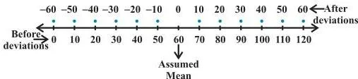
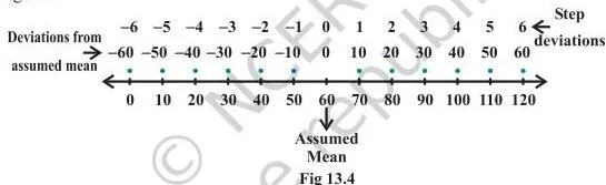
\[ y_i = \frac{x_i – A}{h} \]
Shifting the origin to \(A\) (Fig 13.3) and changing the scale by \(h\) (Fig 13.4) shrink the numbers so the arithmetic gets easier.
Then the mean and variance follow from the step-deviations \(y_i\):
\[ \bar{x} = A + h\frac{\sum f_i y_i}{N}, \qquad \sigma^2 = \frac{h^2}{N^2}\left[N\sum f_i y_i^2 – \left(\sum f_i y_i\right)^2\right] \]
Worked check: classes 20-30, 30-40, 40-50 with frequencies 3, 5, 2. Take \(A = 35\), \(h = 10\). Mid-points are 25, 35, 45, so \(y_i = -1, 0, 1\). Then \(\sum f y = -3 + 0 + 2 = -1\), \(\sum f y^2 = 3 + 0 + 2 = 5\), \(N = 10\). Hence \(\bar{x} = 35 + \frac{-1}{10} \times 10 = 34\) and \(\sigma^2 = \frac{100}{100}(10 \times 5 – 1) = 49\), so \(\sigma = 7\).
Properties of Variance and Standard Deviation
Two transformation rules save a lot of time (NCERT, pp. 283-286):
- Add (or subtract) a constant \(a\) to every observation: the variance and standard deviation stay unchanged, because every deviation \(x_i – \bar{x}\) is untouched.
- Multiply every observation by a constant \(k\): the standard deviation multiplies by \(|k|\) and the variance by \(k^2\).
Example: the variance of 20 observations is 5; if each is multiplied by 2, the new variance is \(2^2 \times 5 = 20\). This is exactly the pattern of NCERT Example 13 (p. 283), where the sum of squared deviations quadrupled from 100 to 400.
A common exam twist asks for two missing observations when the mean and variance are known (Example 14 style, p. 284). Work it in two equations: use the mean to get \(x + y\), then use the variance, expanded as \(\frac{1}{n}(\sum x_i^2 – n\bar{x}^2)\), to get \(x^2 + y^2\). Subtract to find \((x – y)^2\), then solve for \(x\) and \(y\).
Real-life application: standard deviation powers quality control. Suppose a machine fills 200 g packets of biscuits; if the SD of the fill weights is tiny, the machine is consistent and almost every packet is close to 200 g, while a large SD means some packets are seriously under- or overfilled.
Manufacturers set tolerance limits in multiples of \(\sigma\) to decide whether the process is running well. The same idea ranks consistency of batsmen, students or investments.
Limitations of Mean Deviation
NCERT lists three weaknesses (p. 271):
- In a series with very high variability, the median is not a representative central value, so mean deviation about the median loses reliability.
- The sum of absolute deviations from the mean is larger than from the median, which makes mean deviation about the mean less scientific.
- Absolute values cannot be manipulated algebraically, so mean deviation cannot feed into further statistical treatment.
These problems push us to standard deviation, which uses squares and is fully algebraic.
Edge case — median vs mean: when the data contains outliers (a single extreme score), the median is the safer central value for mean deviation because it ignores the extreme’s pull on the centre. Use the mean only when the data is symmetric and free of extreme values.
Definitions: Essential Terms in Table Form
| Term | Meaning | Example |
|---|---|---|
| Dispersion | Scatter or spread of data around a central value | Batsman A’s scores are more dispersed than B’s |
| Range | Maximum value minus minimum value | For batsman A: \(117 – 0 = 117\) |
| Deviation | Difference \(x – a\) between an observation and a fixed value | If mean is 9, the observation 6 has deviation \(-3\) |
| Absolute deviation | Distance \(|x – a|\), the deviation with the sign dropped | \(|6 – 9| = 3\) |
| Mean deviation | Mean of the absolute deviations from a central value | \(\text{M.D.}(\bar{x}) = \frac{1}{n}\sum|x_i – \bar{x}|\) |
| Variance | Mean of the squared deviations from the mean | \(\sigma^2 = \frac{1}{n}\sum(x_i – \bar{x})^2\) |
| Standard deviation | Positive square root of the variance; same units as data | \(\sigma = \sqrt{\sigma^2}\) |
| Median class | Class interval whose cumulative frequency is just \(\geq N/2\) | In the example above, 10-20 |
| Step-deviation | Transformed value \(y_i = (x_i – A)/h\) used in shortcuts | Mid-point 45 with \(A = 35, h = 10\) gives \(y = 1\) |
Formulas You Must Memorise for the Exam
This sheet matches the NC
ERT Summary (pp. 287-288). Symbols: \(N = \sum f_i\), \(M\) = median, \(\bar{x}\) = mean, \(h\) = class width, \(A\) = assumed mean.
| Situation | Formula |
|---|---|
| Range | \(\text{Maximum} – \text{Minimum}\) |
| Mean deviation, ungrouped | \(\text{M.D.}(\bar{x}) = \frac{\sum|x_i – \bar{x}|}{n}\), \(\text{M.D.}(M) = \frac{\sum|x_i – M|}{n}\) |
| Mean deviation, grouped | \(\text{M.D.}(\bar{x}) = \frac{\sum f_i|x_i – \bar{x}|}{N}\), \(\text{M.D.}(M) = \frac{\sum f_i|x_i – M|}{N}\) |
| Variance and SD, ungrouped | \(\sigma^2 = \frac{1}{n}\sum(x_i – \bar{x})^2\), \(\sigma = \sqrt{\sigma^2}\) |
| Variance and SD, discrete | \(\sigma^2 = \frac{1}{N}\sum f_i(x_i – \bar{x})^2\) |
| Variance and SD, continuous | \(\sigma = \frac{1}{N}\sqrt{N\sum f_i x_i^2 – (\sum f_i x_i)^2}\) |
| Step-deviation mean | \(\bar{x} = A + h\frac{\sum f_i y_i}{N}\), where \(y_i = \frac{x_i – A}{h}\) |
| Step-deviation variance | \(\sigma^2 = \frac{h^2}{N^2}[N\sum f_i y_i^2 – (\sum f_i y_i)^2]\) |
| Median (grouped) | \(l + \frac{\frac{N}{2} – C}{f} \times h\) |
Worked Examples: Step-by-Step to Full Marks
Example 1: Mean deviation about the mean for ungrouped data
Find \(\text{M.D.}(\bar{x})\) for 3, 8, 12, 15, 7, 10.
Step 1: Compute the mean. \(\bar{x} = \frac{3+8+12+15+7+10}{6} = \frac{55}{6} = 9.17\).
Step 2: Find absolute deviations \(|x_i – \bar{x}|\): \(|3-9.17| = 6.17\), \(|8-9.17| = 1.17\), \(|12-9.17| = 2.83\), \(|15-9.17| = 5.83\), \(|7-9.17| = 2.17\), \(|10-9.17| = 0.83\).
Step 3: Sum them: \(6.17 + 1.17 + 2.83 + 5.83 + 2.17 + 0.83 = 19.00\).
Step 4: \(\text{M.D.}(\bar{x}) = \frac{19}{6} = 3.17\).
Final answer: \(\text{M.D.}(\bar{x}) = 3.17\).
Example 2: Mean deviation about the median for continuous data
Classes 0-10, 10-20, 20-30 with frequencies 4, 6, 5.
Step 1: \(N = 15\), so \(N/2 = 7.5\). Cumulative frequencies: 4, 10, 15. The class 10-20 is the median class.
Step 2: Median \(= 10 + \frac{7.5 – 4}{6} \times 10 = 10 + 5.83 = 15.83\).
Step 3: Mid-points are 5, 15, 25. Absolute deviations from 15.83: \(|5-15.83| = 10.83\), \(|15-15.83| = 0.83\), \(|25-15.83| = 9.17\).
Step 4: \(\sum f_i|x_i – M| = 4(10.83) + 6(0.83) + 5(9.17) = 43.32 + 4.98 + 45.85 = 94.15\).
Step 5: \(\text{M.D.}(M) = \frac{94.15}{15} = 6.28\).
Final answer: \(\text{M.D.}(M) = 6.28\).
Example 3: Variance and standard deviation of a discrete distribution
For \(x = 5, 10, 15, 20\) with frequencies 2, 5, 3, 1:
Step 1: \(N = 2+5+3+1 = 11\).
Step 2: \(\sum f x = 2(5) + 5(10) + 3(15) + 1(20) = 10 + 50 + 45 + 20 = 125\).
Step 3: \(\sum f x^2 = 2(25) + 5(100) + 3(225) + 1(400) = 50 + 500 + 675 + 400 = 1625\).
Step 4: \(\sigma^2 = \frac{1}{N}[\sum f x^2 – \frac{(\sum f x)^2}{N}] = \frac{1}{11}[1625 – \frac{15625}{11}] = \frac{2250}{121} = 18.60\).
Step 5: \(\sigma = \sqrt{18.60} = 4.31\).
Final answer: variance \(= 18.60\), standard deviation \(= 4.31\).
Common Mistakes Students Make in Statistics
| Mistake | Correct rule | How to check your answer |
|---|---|---|
| Writing \(\sum(x_i – \bar{x})\) instead of \(\sum|x_i – \bar{x}|\) in mean deviation | Mean deviation always uses absolute values; the raw sum is 0 | If your deviation sum is zero, you forgot the absolute value signs |
| Using \(n\) instead of \(N = \sum f_i\) for grouped data | Grouped formulas divide by the total frequency \(N\) | Count the frequencies; the denominator must be their total |
| Not squaring deviations in variance | Variance squares each deviation before averaging | Variance can never be negative; a negative answer means a squaring error |
| Picking the wrong median class | Median class = interval whose cumulative frequency is just \(\geq N/2\) | Write the cumulative frequency column first |
| Forgetting to multiply by \(h\) in the step-deviation mean | \(\bar{x} = A + h\frac{\sum f_i y_i}{N}\) includes the class width | Sanity-check: the mean must lie inside the data range |
| Confusing variance and standard deviation | Variance is \(\sigma^2\); standard deviation is \(\sigma = \sqrt{\sigma^2}\) | Read the question again — did it ask for variance or SD? |
Misconception autopsy: variance and standard deviation are not interchangeable. They measure the same spread but on different scales — variance is in squared units, SD is in the original units. If the data is heights in cm, the variance is in cm² while the SD is in cm.
Quoting one when the other is asked loses the mark even if your table is perfect.
Exam Notes: How to Score Marks in This Chapter
- Marks are typically awarded in three visible chunks: writing the correct formula, building the computation table (including cumulative frequency for medians), and substituting numbers correctly. A formula quoted but never used earns nothing.
- Mean deviation about the mean or median for grouped data is a frequently set question — rehearse the full table layout so you can produce it fast under time pressure.
- The step-deviation method is accepted as a time-saver when you choose \(A\) and \(h\) correctly. Pick \(A\) as a mid-point near the centre and \(h\) as the common class width; a wrong \(A\) or \(h\) invalidates every later step.
- Property problems (variance unchanged when a constant is added; multiplied by \(k^2\) when data is scaled by \(k\)) can appear as short, analytical questions — state the rule and apply it, do not re-derive it from scratch.
- Mixed problems that combine mean and variance, such as finding two missing observations, reward clean equation framing: one equation from the mean, one from the variance, then solve.
Quick Revision: Statistics Class 11 Notes on One Page
| Measure | Formula (ungrouped) | Formula (grouped) | Use |
|---|---|---|---|
| Range | \(\max – \min\) | \(\max – \min\) | Rough first idea of spread |
| Mean deviation | \(\frac{1}{n}\sum|x_i – a|\) | \(\frac{1}{N}\sum f_i|x_i – a|\) | Average distance from centre |
| Standard deviation | \(\sqrt{\frac{1}{n}\sum(x_i – \bar{x})^2}\) | \(\frac{1}{N}\sqrt{N\sum f_i x_i^2 – (\sum f_i x_i)^2}\) | Precise spread, same units as data |
- Use range for a quick comparison, mean deviation when you want the average distance from a centre, and standard deviation when you need precision or further statistical work.
- Memory aid: SD is the root mean square of the deviations — square, average, root.
- Adding a constant does not change the SD; multiplying by \(k\) multiplies the SD by \(|k|\) and the variance by \(k^2\).
- Mean deviation uses absolute values; variance and SD use squares — that is the central design choice of this chapter.
Figure Walkthrough: Reading the Diagrams
Four sets of diagrams carry the chapter’s intuition, and all are shown above in their sections.
- Batsmen dots (Figs 13.1-13.2): when values are plotted as dots on one line, dispersion becomes visible. A’s dots stretch from 0 to 117; B’s pile up around 53. Two data sets with equal means can look completely different — that is the motivation for the whole chapter (p. 259).
- Shifting origin (Fig 13.3): subtracting the assumed mean from each value slides every point left, shrinking the numbers without changing the gaps between them.
- Changing scale (Fig 13.4): dividing each shift by the common factor \(h\) compresses the scale further, giving tidy step-deviations like \(-1, 0, 1\) (pp. 267-268).
- Set A vs set B (Figs 13.5-13.6): A’s six dots run from deviation \(-25\) to \(+25\); B’s 31 dots run only from \(-15\) to \(+15\). Averaging the squared deviations, not summing them, correctly ranks A as more scattered (pp. 273-274).
Frequently Asked Questions about Statistics Class 11 Notes
Why do we use absolute values in mean deviation?
Deviations from the mean sum to zero, so their raw average is always zero and carries no information. Taking absolute values turns each deviation into a distance, so the average is a genuine positive measure of spread.
When should I use median instead of mean for mean deviation?
Use the median when the data has outliers or is highly skewed, because the median ignores the pull of extreme values. Use the mean when the data is symmetric and free of outliers; NCERT notes that the median loses representativeness in very variable data (p. 271).
How do I find the median class in a continuous frequency distribution?
Find \(N/2\), then locate the class whose cumulative frequency is just greater than or equal to \(N/2\). That interval is the median class; feed its \(l, f, h\) and the preceding cumulative frequency \(C\) into the median formula.
What is the difference between variance and standard deviation?
Variance is the mean of the squared deviations; standard deviation is its positive square root. They measure the same spread, but variance is in squared units while SD is in the original units of the data.
Does adding a constant to every observation change the standard deviation?
No. Adding (or subtracting) a constant shifts the whole data set and the mean by the same amount, so every deviation \(x_i – \bar{x}\) and hence the variance and SD remain unchanged (NCERT, p. 285).
How to choose the assumed mean and class width in the step-deviation method?
Choose \(A\) as a mid-point near the centre of the data and \(h\) as the common class width. This produces small integer step-deviations like \(-1, 0, 1\), which keep the multiplication simple and reduce rounding errors.
Reference: NCERT Class 11 Mathematics textbook, chapter 13 Statistics.
Explore Class 11 Mathematics Notes
- Previous: Limits and Derivatives
- Next: Probability
More for this chapter:
Class 11 Mathematics on LearnCBSE:
Related chapters:
- Sets notes
- Relations and Functions notes
- Trigonometric Functions notes
Official source: download the NCERT textbook free from ncert.nic.in.