Here are the Statistics Class 11 formulas you need for this chapter: range, mean deviation, variance and standard deviation, plus the mean, median and step-deviation formulas they build on. The sheet covers ungrouped data, discrete frequency distributions and continuous (class-interval) data.
Each formula is grouped by topic with a symbol table, when-to-use guidance, and three worked examples using fresh numbers. This is a lookup sheet, not a lesson — the derivations belong in the chapter notes. When you revise another chapter, the Class 11 Maths formulas hub collects the formula sheets by chapter so you can jump straight to the next topic.
Formulas at a Glance
This table is the page’s quick index. Every row below is explained in the grouped list that follows.
| Purpose | Formula |
|---|---|
| Mean of a raw data list | \( \bar{x} = \frac{1}{n}\sum_{i=1}^{n} x_i \) |
| Range — quick spread between extremes | \( \text{Range} = \text{Maximum value} – \text{Minimum value} \) |
| Mean deviation about the mean (ungrouped) | \( \text{M.D.}(\bar{x}) = \frac{1}{n}\sum_{i=1}^{n} |x_i – \bar{x}| \) |
| Mean deviation about the median (ungrouped) | \( \text{M.D.}(M) = \frac{1}{n}\sum_{i=1}^{n} |x_i – M| \) |
| Mean of a discrete frequency distribution | \( \bar{x} = \frac{\sum_{i=1}^{n} f_i x_i}{N} \), where \( N = \sum_{i=1}^{n} f_i \) |
| Mean deviation for grouped data (about the mean or median) | \( \text{M.D.}(\bar{x}) = \frac{\sum_{i=1}^{n} f_i |x_i – \bar{x}|}{N} \), \( \text{M.D.}(M) = \frac{1}{N}\sum_{i=1}^{n} f_i |x_i – M| \) |
| Median of a continuous frequency distribution | \( \text{Median} = l + \frac{\frac{N}{2} – C}{f} \times h \) |
| Mean by step-deviation method (large values) | \( d_i = \frac{x_i – a}{h} \), \( \bar{x} = a + \frac{\sum_{i=1}^{n} f_i d_i}{N} \times h \) |
| Variance and standard deviation (ungrouped) | \( \sigma^2 = \frac{1}{n}\sum_{i=1}^{n} (x_i – \bar{x})^2 \), \( \sigma = \sqrt{\frac{1}{n}\sum_{i=1}^{n} (x_i – \bar{x})^2} \) |
| Variance of a discrete frequency distribution | \( \sigma^2 = \frac{1}{N}\sum_{i=1}^{n} f_i (x_i – \bar{x})^2 \) |
| Standard deviation using sums of squares (grouped) | \( \sigma = \frac{1}{N}\sqrt{N\sum_{i=1}^{n} f_i x_i^2 – \left(\sum_{i=1}^{n} f_i x_i\right)^2} \) |
| Standard deviation using sums of squares (ungrouped) | \( \sigma = \sqrt{\frac{1}{n}\sum_{i=1}^{n} x_i^2 – (\bar{x})^2} \) |
| Standard deviation by shortcut (step-deviation) method | \( \sigma = \frac{h}{N}\sqrt{N\sum_{i=1}^{n} f_i y_i^2 – \left(\sum_{i=1}^{n} f_i y_i\right)^2} \), with \( y_i = \frac{x_i – A}{h} \) |
| New variance when every observation is multiplied by \( k \) | \( \sigma^2_{\text{new}} = k^2 \sigma^2 \) (new \( \sigma = |k|\sigma \), new mean \( = k\bar{x} \)) |
| Variance when a constant is added to every observation | \( \sigma^2_{\text{new}} = \sigma^2 \) |
All Formulas, Grouped by Topic
Range
The range is the difference between the maximum and minimum values of a series. It uses only the two extremes, so it gives a rough idea of scatter, not a picture of how the data sits around a central value (NCERT, p. 287).
\[ \text{Range} = \text{Maximum value} – \text{Minimum value} \]
The chapter opens with two batsmen whose mean and median are both 53, yet whose performances look very different. The dot plots below show why: A’s scores scatter from 0 to 117, while B’s cluster between 46 and 60 (NCERT, p. 258). Range turns this difference into a single number.


Mean Deviation for Ungrouped Data
A deviation is the difference \( x_i – a \). The mean deviation about a central value \( a \) is the mean of the absolute deviations of the observations from \( a \) (NCERT, p. 260). The absolute-value signs are essential: the sum of the signed deviations from the mean is always zero, so without them every mean deviation would come out 0.
\[ \text{M.D.}(a) = \frac{1}{n}\sum_{i=1}^{n} |x_i – a| \]
Putting \( a = \bar{x} \) (the mean) or \( a = M \) (the median) gives the two standard forms (NCERT, p. 261):
\[ \text{M.D.}(\bar{x}) = \frac{1}{n}\sum_{i=1}^{n} |x_i – \bar{x}|, \qquad \text{M.D.}(M) = \frac{1}{n}\sum_{i=1}^{n} |x_i – M| \]
For M.D.(M) you first need the median. In a raw list arranged in order, for odd \( n \) the median is the \( \left(\frac{n+1}{2}\right) \)th observation; for even \( n \) it is the mean of the \( \frac{n}{2} \)th and \( \left(\frac{n}{2}+1\right) \)th observations (NCERT, p. 258).
Mean Deviation for Grouped Data
For a discrete frequency distribution, each value \( x_i \) occurs with frequency \( f_i \). Find the mean first, then weight every absolute deviation by its frequency (NCERT, §13.4.2):
\[ \bar{x} = \frac{\sum_{i=1}^{n} f_i x_i}{N}, \qquad N = \sum_{i=1}^{n} f_i \]
\[ \text{M.D.}(\bar{x}) = \frac{\sum_{i=1}^{n} f_i |x_i – \bar{x}|}{N}, \qquad \text{M.D.}(M) = \frac{1}{N}\sum_{i=1}^{n} f_i |x_i – M| \]
For continuous (class-interval) data, replace each class by its mid-point and use the same formulas — the frequency of a class is taken to be centred at its mid-point (NCERT, p. 266).
For M.D. about the median you need the median of the continuous data. Locate the median class — the class whose cumulative frequency is just greater than or equal to \( \frac{N}{2} \) — then interpolate inside it (NCERT, p. 269):
\[ \text{Median} = l + \frac{\frac{N}{2} – C}{f} \times h \]
Mean by Step-Deviation Method
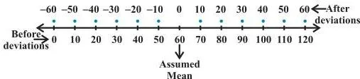
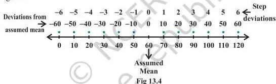
When the values or mid-points are large, shift the origin to an assumed mean \( a \) and divide by a common factor \( h \). This shrinks the arithmetic without changing the final mean (NCERT, p. 268). The two moves are a change of origin (Fig 13.3) and a change of scale (Fig 13.4).
\[ d_i = \frac{x_i – a}{h}, \qquad \bar{x} = a + \frac{\sum_{i=1}^{n} f_i d_i}{N} \times h \]
Variance and Standard Deviation
Mean deviation is built on absolute values, which are hard to handle algebraically. Squaring the deviations removes the signs instead. The mean of the squared deviations is the variance \( \sigma^2 \); its positive square root is the standard deviation \( \sigma \) (NCERT, p. 274).
\[ \sigma^2 = \frac{1}{n}\sum_{i=1}^{n} (x_i – \bar{x})^2, \qquad \sigma = \sqrt{\frac{1}{n}\sum_{i=1}^{n} (x_i – \bar{x})^2} \]
Why divide by \( n \)? The plain sum of squared deviations favours larger data sets. In the chapter’s comparison, both sets have mean 30, but the set of 31 observations gives the larger sum (2480 against 1750) even though it is less scattered. Dividing by \( n \) reverses the verdict, which is why variance averages the squares (NCERT, p. 273). The plots below show the two sets.


For a discrete frequency distribution, weight each squared deviation by its frequency (NCERT, p. 287):
\[ \sigma^2 = \frac{1}{N}\sum_{i=1}^{n} f_i (x_i – \bar{x})^2 \]
For a continuous distribution, use the class mid-points as the \( x_i \) in the same formula.
Expanding the square and simplifying leads to a working form that avoids computing every deviation (NCERT, p. 278):
\[ \sigma^2 = \frac{1}{N}\sum_{i=1}^{n} f_i x_i^2 – \left( \frac{\sum_{i=1}^{n} f_i x_i}{N} \right)^2, \qquad \sigma = \frac{1}{N}\sqrt{N\sum_{i=1}^{n} f_i x_i^2 – \left( \sum_{i=1}^{n} f_i x_i \right)^2} \]
The ungrouped version of the same idea, used when a data set is corrected, is \( \sigma = \sqrt{ \frac{1}{n}\sum_{i=1}^{n} x_i^2 – (\bar{x})^2 } \) (NCERT, Example 16).
Shortcut Method for Variance and Standard Deviation
When the values or mid-points are large and every class has the same width \( h \), take step-deviations \( y_i \) about an assumed mean \( A \). Because each \( x_i \) is a scaled, shifted version of \( y_i \), the standard deviation of \( x \) is \( h \) times the standard deviation of \( y \) (NCERT, p. 280):
\[ y_i = \frac{x_i – A}{h}, \qquad \bar{x} = A + h\bar{y}, \qquad \sigma_x = h\sigma_y \]
The working formula for the standard deviation is \[ \sigma = \frac{h}{N}\sqrt{N\sum_{i=1}^{n} f_i y_i^2 – \left( \sum_{i=1}^{n} f_i y_i \right)^2} \]
The variance is the square of this: \( \sigma^2 = \frac{h^2}{N^2}\left[ N\sum_{i=1}^{n} f_i y_i^2 – \left( \sum_{i=1}^{n} f_i y_i \right)^2 \right] \). The shortcut needs one uniform width \( h \) for all classes.
Scaling and Shifting Data (Miscellaneous Examples)
Two results from the miscellaneous examples answer whole questions in one step. If every observation is multiplied by \( k \), the variance becomes \( k^2 \) times the original variance (NCERT, p. 283):
\[ \sigma^2_{\text{new}} = k^2 \sigma^2 \]
Since \( \sigma \) is the positive square root of the variance, the new standard deviation is \( |k| \sigma \), and the new mean is \( k\bar{x} \).
Adding (or subtracting) a constant to every observation does not affect the variance, because each deviation \( x_i – \bar{x} \) is unchanged (NCERT, p. 285):
\[ \sigma^2_{\text{new}} = \sigma^2 \]
What Each Symbol Means
Read the symbols column by column: the letter in the formula, what it names in the data, and what unit it carries.
| Symbol | What it means | Unit / nature |
|---|---|---|
| \( x_i \) | The \( i \)-th observation (or class mid-point) | Same unit as the data — marks, cm, kg, ₹, runs |
| \( n \) | Number of observations in ungrouped data | A count — no unit |
| \( f_i \) | Frequency of the \( i \)-th value or class | A count — no unit |
| \( N = \sum f_i \) | Total frequency of a distribution | A count — no unit |
| \( \bar{x} \) | Arithmetic mean of the data | Same unit as the data |
| \( M \) | Median of the data; this chapter uses \( M \) for the median | Same unit as the data |
| \( a \) | Central value used for mean deviation (usually \( \bar{x} \) or \( M \)); also the assumed mean in the step-deviation method | Same unit as the data |
| \( |x_i – a| \) | Absolute deviation — the distance of \( x_i \) from \( a \) | Same unit as the data |
| \( l \) | Lower limit of the median class | Same unit as the data |
| \( C \) | Cumulative frequency of the class just before the median class | A count — no unit |
| \( f \) | Frequency of the median class | A count — no unit |
| \( h \) | Width of a class interval | Same unit as the data |
| \( A \) | Assumed mean in the shortcut method | Same unit as the data |
| \( d_i ,\ y_i \) | Step-deviations \( (x_i – a)/h \) or \( (x_i – A)/h \) | A ratio — no unit |
| \( \bar{y} \) | Mean of the step-deviations \( y_i \) | A ratio — no unit |
| \( \sigma^2 \) | Variance — the mean of squared deviations | Square of the data unit (marks², cm²) |
| \( \sigma \) | Standard deviation — positive square root of the variance | Same unit as the data |
This unit pattern is a built-in check: \( \sigma \) carries the unit of the data (so 3.87 cm makes sense for heights), while \( \sigma^2 \) carries the squared unit. That is why the chapter presents \( \sigma \) as the practical measure of dispersion (NCERT, p. 274).
When to Use Each Formula
| Formula | Reach for it when… | Condition to check |
|---|---|---|
| \( \bar{x} = \frac{1}{n}\sum x_i \) | You need the central value of a raw list. | Data is ungrouped. |
| Range | You want the overall span in one number. | Only the extremes matter; the middle values are ignored. |
| \( \text{M.D.}(\bar{x}) \), \( \text{M.D.}(M) \) | Data is a raw list and the question asks for mean deviation about the mean or median. | Use the absolute deviation \( |x_i – a| \), never the signed deviation. |
| Grouped M.D. formulas | Data is a discrete frequency table, or classes with frequencies. | For classes, replace each class by its mid-point first. |
| Median formula | Data is continuous and you need the median (for M.D. about median). | Median class = the class whose cumulative frequency first reaches or passes \( \frac{N}{2} \); \( C \) is the cumulative frequency before it. |
| Step-deviation mean | Values or mid-points are large and classes share one width. | Pick \( a \) near the centre; use the same \( h \) for every class. |
| Variance / SD formulas | You need the standard measure of scatter, not the rough range. | \( \sigma \) carries the data’s unit; variance carries its square. |
| Sums-of-squares form of SD | You want to avoid decimals from \( (x_i – \bar{x}) \) and already have columns for \( f_i x_i \) and \( f_i x_i^2 \). | Build \( \sum f_i x_i^2 \) and \( (\sum f_i x_i)^2 \) in separate columns. |
| Shortcut SD with \( y_i \) | Large values or mid-points with a uniform class width \( h \). | Use one assumed mean \( A \); the same \( h \) for all classes. |
| \( k^2\sigma^2 \), \( k\bar{x} \) | Every observation is multiplied by the same constant (for example, converting units). | Variance scales by \( k^2 \), SD by \( |k| \), mean by \( k \). |
| Variance unchanged by shift | A constant is added to (or subtracted from) every observation. | Only the mean shifts; variance and SD stay as they were. |
Worked Examples
Three original problems that use the formulas the way the exam does. Each shows the formula being selected, the substitution, and the answer with its unit.
Worked Example 1: Mean deviation about the mean (ungrouped)
Find the mean deviation about the mean for the marks 5, 8, 10, 14, 18, scored out of 20 in five tests.
Step 1 — select the formula.
Data is ungrouped and the central value is \( \bar{x} \), so use \( \text{M.D.}(\bar{x}) = \frac{1}{n}\sum |x_i – \bar{x}| \).
Step 2 — find the mean.
\[ \bar{x} = \frac{5 + 8 + 10 + 14 + 18}{5} = \frac{55}{5} = 11 \]
Step 3 — take absolute deviations.
\[ |5-11|, |8-11|, |10-11|, |14-11|, |18-11| = 6,\ 3,\ 1,\ 3,\ 7 \]
Step 4 — average the distances.
\[ \text{M.D.}(\bar{x}) = \frac{6 + 3 + 1 + 3 + 7}{5} = \frac{20}{5} = 4 \]
Final answer: the mean deviation about the mean is 4 marks.
Worked Example 2: Finding missing observations from the mean and variance
The mean and variance of five observations are 10 and 16.4. Three of the observations are 6, 10 and 14. Find the remaining two.
Step 1 — use the mean.
Total of all five observations is \( 5 \times 10 = 50 \).
The known observations total \( 6 + 10 + 14 = 30 \), so the missing pair satisfies \( x + y = 20 \).
Step 2 — use the variance.
From \( \sigma^2 = \frac{1}{n}\sum (x_i – \bar{x})^2 \), the total sum of squared deviations is \( n\sigma^2 = 5 \times 16.4 = 82 \).
The known observations contribute \( (-4)^2 + 0^2 + 4^2 = 32 \), so the missing pair must satisfy \( (x – 10)^2 + (y – 10)^2 = 50 \).
Step 3 — solve.
Put \( u = x – 10 \) and \( v = y – 10 \).
Then \( u + v = 0 \) and \( u^2 + v^2 = 50 \), which gives \( u = 5 \), \( v = -5 \) (or vice versa).
So \( x = 15 \) and \( y = 5 \).
Final answer: the missing observations are 5 and 15. Check: mean \( = 50/5 = 10 \), and variance \( = \frac{16 + 0 + 16 + 25 + 25}{5} = 16.4 \).
Worked Example 3: Variance and standard deviation of a discrete frequency distribution
Marks \( x_i \): 4, 8, 12, 16 with frequencies \( f_i \): 5, 10, 15, 10. Find the variance and standard deviation of the distribution.
Step 1 — select the formula.
Use the sums-of-squares form so no individual deviation is needed: \( \sigma^2 = \frac{1}{N}\sum f_i x_i^2 – \left( \frac{\sum f_i x_i}{N} \right)^2 \).
Step 2 — build the sums.
\[ N = 40, \qquad \sum f_i x_i = 5(4) + 10(8) + 15(12) + 10(16) = 440 \]
\[ \sum f_i x_i^2 = 5(16) + 10(64) + 15(144) + 10(256) = 5440 \]
Step 3 — substitute.
\[ \sigma^2 = \frac{5440}{40} – \left( \frac{440}{40} \right)^2 = 136 – 121 = 15 \]
Step 4 — take the positive square root.
\[ \sigma = \sqrt{15} = 3.87 \]
Check.
Direct deviations from the mean 11 give \( \sum f_i (x_i – 11)^2 = 245 + 90 + 15 + 250 = 600 \), and \( 600/40 = 15 \) — the same variance.
Final answer: variance \( = 15 \) marks² and standard deviation \( \approx 3.87 \) marks.
Common Mistakes to Avoid
These are the errors this chapter’s formulas invite. Each row gives the correction and a one-line check you can run on your own answer.
| Mistake | Correct rule | How to check your answer |
|---|---|---|
| Dropping the absolute-value signs in mean deviation | Sum \( |x_i – a| \) first, then divide by \( n \). The signed sum \( \sum (x_i – \bar{x}) \) is always zero (NCERT, p. 260). | If your M.D. is 0 for mixed data, you forgot the modulus. |
| Mixing \( \sum f_i x_i^2 \) with \( (\sum f_i x_i)^2 \) in the sums-of-squares formula | Keep them in separate columns; the root contains \( N\sum f_i x_i^2 – (\sum f_i x_i)^2 \). | The bracket inside the root equals \( N\left( \frac{\sum f_i x_i^2}{N} – \bar{x}^2 \right) \), which must be non-negative. |
| Stopping at variance when the question asks for standard deviation | \( \sigma = \sqrt{\sigma^2} \), the positive root. Variance is \( \sigma^2 \); standard deviation is \( \sigma \). | \( \sigma \) has the same unit as the data; if your answer carries a squared unit, it is the variance. |
| Using the median class’s own cumulative frequency as \( C \) | \( C \) is the cumulative frequency of the class just before the median class. | The computed median must lie inside the median class, between \( l \) and \( l + h \). |
| Using class intervals that have gaps between them | Make the data continuous first: subtract 0.5 from each lower limit and add 0.5 to each upper limit (chapter hint, Exercise 13.1). | The upper boundary of one class must equal the lower boundary of the next. |
Frequently Asked Questions
What is the difference between variance and standard deviation?
Variance \( \sigma^2 \) is the mean of the squared deviations of the observations from their mean. Standard deviation \( \sigma \) is its positive square root (NCERT, p. 274). Because the square root cancels the squaring, \( \sigma \) has the same unit as the data, which makes it the practical measure of dispersion.
Why does mean deviation use absolute values?
Because the sum of the signed deviations from the mean is always zero — positive and negative deviations cancel. Taking absolute values converts every deviation into a distance, so their mean measures spread instead of cancelling out (NCERT, p. 260).
When should I use the step-deviation (shortcut) method?
When the observations or class mid-points are large and all class widths are equal. Choose an assumed mean \( a \) (or \( A \)) and a common factor \( h \), work with \( d_i = (x_i – a)/h \) or \( y_i = (x_i – A)/h \), then multiply back. The mean and standard deviation come out identical to the direct method (NCERT, pp. 268, 280).
Does adding or multiplying by a constant change the variance?
Adding (or subtracting) a constant leaves the variance unchanged, because every deviation \( x_i – \bar{x} \) is untouched. Multiplying every observation by \( k \) multiplies the variance by \( k^2 \), the standard deviation by \( |k| \), and the mean by \( k \) (NCERT, pp. 283–285).
Revising other chapters? The Maths formulas collection holds the formula sheets for the rest of the Class 11 course.
Reference: NCERT Class 11 Mathematics textbook, chapter Statistics.
Verify any formula against the official Rationalised NCERT Class 11 Mathematics textbook (chapter 13, Statistics) at ncert.nic.in.
Explore Class 11 Maths Formulas
More for this chapter:
- Statistics Notes
Related chapters: