These probability class 11 notes condense Chapter 14 of the NCERT Class 11 Mathematics textbook into revision-ready form: definitions, the three axioms, the counting formula, the addition theorem and the complement rule, with worked examples throughout. Revise in the order given below — each section assumes the one before it. The notes follow the 2026-27 rationalised NCERT edition.
Use this page the night before a class test: read the tables, work the three solved examples on paper, then scan the common-mistakes and exam-notes sections. If a definition or formula is unclear, open the official NCERT Class 11 Mathematics Chapter 14 PDF for the full treatment.
Probability Class 11 Notes: What to Revise and in What Order
Probability in Class 11 is a chain — every idea sits on the one before it. Build it in this order:
- Random experiment and sample space — the set \(S\) of all possible outcomes.
- Event — any subset \(E\) of \(S\).
- Algebra of events — union, intersection, difference and complement applied to events.
- Types of events — impossible, sure, simple, compound, mutually exclusive, exhaustive.
- Axiomatic probability — the three axioms plus the two validity checks.
- Equally likely outcomes — the counting formula \(P(E) = \frac{n(E)}{n(S)}\).
- Addition theorem and complement — the two rules nearly every numerical uses.
Two earlier chapters do the heavy lifting: Set language is the algebra of events in disguise, and counting supplies \(n(S)\) and \(n(E)\). If a probability problem feels hard, the difficulty is usually the counting. Brush up with the Class 11 Sets notes and Permutations and Combinations notes before attempting Exercise 14.2.
The three exercise sets test this material in a deliberate sequence:
- Exercise 14.1 — describing events, the algebra of events, and mutually exclusive / exhaustive checks.
- Exercise 14.2 — valid probability assignments, \(P(A \cup B)\), \(P(A’)\), and equally likely counting problems.
- Miscellaneous Exercise — combined problems that join probability with combinations and permutations, plus the three-event formula.
For the bigger picture, see the Class 11 Mathematics notes hub, the Class 11 hub and the CBSE notes home.
Key Probability Terms in One Table
Every definition in this chapter is a set statement. Scan this table first; it holds the vocabulary for everything that follows (NCERT, pp. 290–294).
| Term | Meaning | Example |
|---|---|---|
| Sample space | The set of all possible outcomes of a random experiment. | Tossing two coins: \(S = \{HH, HT, TH, TT\}\) |
| Event | Any subset \(E\) of the sample space \(S\). | \(E = \{HT, TH\}\) is ‘exactly one head’ |
| Impossible event | The empty set \(\phi\) — no outcome can make it occur. | ‘Multiple of 7 on a die’ is \(\phi\) |
| Sure event | The whole sample space \(S\) — every outcome makes it occur. | ‘Odd or even number on a die’ is \(S\) |
| Simple event | An event with exactly one sample point. | \(\{HH\}\) in a two-coin toss |
| Compound event | An event with more than one sample point. | \(\{HT, TH\}\) |
| Complementary event | \(A’ = S – A\), all outcomes of \(S\) that are not in \(A\). | If \(A = \{HH\}\), then \(A’ = \{HT, TH, TT\}\) |
| Mutually exclusive events | \(A \cap B = \phi\) — they cannot occur together. | ‘Odd’ and ‘even’ on a die |
| Exhaustive events | The union of the events equals \(S\) — at least one must occur. | \(\{1,2,3\}\), \(\{3,4\}\), \(\{5,6\}\) for a die |
Event: The Building Block of Probability
An event is any subset \(E\) of the sample space \(S\) (NCERT, p. 290). A description of a happening becomes a set by collecting exactly the outcomes that satisfy it. In the two-coin experiment \(S = \{HH, HT, TH, TT\}\):
- ‘Number of tails is exactly 2’ gives \(A = \{TT\}\)
- ‘At least one tail’ gives \(B = \{HT, TH, TT\}\)
- ‘Number of heads is at most one’ gives \(C = \{HT, TH, TT\}\)
- ‘Number of tails is more than two’ gives \(\phi\), the impossible event
Occurrence: the event \(E\) has occurred if the outcome \(\omega\) of the experiment satisfies \(\omega \in E\). If \(\omega \notin E\), the event has not occurred (NCERT, p. 291).
Because each sample point can form its own singleton set, a sample space with \(n\) elements has exactly \(n\) simple events — one for each outcome.
Algebra of Events: Combining Events With Sets
Every everyday phrase about events translates into a set operation. Learn the translation once; the formulas later are just set expressions in disguise.
| Event language | Set notation | Meaning |
|---|---|---|
| not A | \(A’ = S – A\) | Complement: outcomes not in A |
| A or B | \(A \cup B\) | Union: outcomes in A, in B, or in both |
| A and B | \(A \cap B\) | Intersection: outcomes in both |
| A but not B | \(A – B = A \cap B’\) | Difference: outcomes in A only |
Work one original example on a die. Take \(S = \{1,2,3,4,5,6\}\), \(A\) = ‘prime’ = \(\{2,3,5\}\), \(B\) = ‘odd’ = \(\{1,3,5\}\). Then:
- \(A \cup B = \{1,2,3,5\}\)
- \(A \cap B = \{3,5\}\)
- \(A – B = \{2\}\)
- \(A’ = \{1,4,6\}\)
De Morgan’s law \(A’ \cap B’ = (A \cup B)’\) turns ‘neither A nor B’ into ‘not A and not B’. Example 7 on page 305 uses exactly this step to find the probability that both students fail.
Mutually Exclusive vs Exhaustive Events
These two classifications are independent. Test them separately:
- Mutually exclusive: \(A \cap B = \phi\). The events share no outcome, so they cannot occur together (NCERT, p. 293).
- Exhaustive: \(E_1 \cup E_2 \cup \dots \cup E_n = S\). At least one of them must occur every time the experiment is run (NCERT, p. 294).
- Mutually exclusive and exhaustive: both conditions at once — the events are pairwise disjoint and their union is \(S\).
The classic three-coin example (NCERT, p. 294). Toss a coin three times; let A = ‘no head’, B = ‘exactly one head’, C = ‘at least two heads’:
- \(A = \{TTT\}\), \(B = \{HTT, THT, TTH\}\), \(C = \{HHT, HTH, THH, HHH\}\)
- Pairwise intersections are empty: \(A \cap B = \phi\), \(A \cap C = \phi\), \(B \cap C = \phi\) — mutually exclusive
- \(A \cup B \cup C = S\) — exhaustive
Counter-example: on a die, ‘odd’ = \(\{1,3,5\}\) and ‘less than 4’ = \(\{1,2,3\}\) are not mutually exclusive because 3 lies in both. Also remember the remark on page 293: simple events of a sample space are always mutually exclusive.
Axiomatic Approach: Three Axioms, Two Checks
Probability is a function P that assigns a real number to every event. The three axioms (NCERT, pp. 296–297) are the rules every valid assignment must obey:
- \(P(E) \geq 0\) for every event \(E\) — no probability is negative.
- \(P(S) = 1\) — the sure event has probability 1.
- If \(E\) and \(F\) are mutually exclusive, \(P(E \cup F) = P(E) + P(F)\) — probabilities of disjoint events add.
Taking \(F = \phi\) in axiom (iii) gives \(P(E \cup \phi) = P(E) + P(\phi)\), so \(P(\phi) = 0\) — the impossible event has probability zero.
The two-check method for any assignment — the fast route to Exercise 14.2 Q1. An assignment of probabilities to outcomes \(\omega_1, \omega_2, \dots, \omega_n\) is valid if and only if:
- \(0 \leq P(\omega_i) \leq 1\) for every outcome, and
- \(P(\omega_1) + P(\omega_2) + \dots + P(\omega_n) = 1\).
Then for any event \(A\), \(P(A) = \sum P(\omega_i)\) over all \(\omega_i \in A\) — add the probabilities of the sample points inside \(A\). The singleton \(\{\omega_i\}\) is the elementary event, and \(P(\omega_i)\) is shorthand for \(P(\{\omega_i\})\) (NCERT, p. 297).
Why do we need axioms at all? Because probability is not forced to be unique. For a coin toss, both \(P(H) = \frac{1}{2}, P(T) = \frac{1}{2}\) and \(P(H) = \frac{1}{4}, P(T) = \frac{3}{4}\) are valid assignments — each satisfies the two checks (NCERT, p. 297).
In general, any \(p\) with \(0 \leq p \leq 1\) works: \(P(H) = p\) and \(P(T) = 1 – p\). The classical formula gives a unique answer only when you add the fairness assumption.
| Classical approach | Axiomatic approach | |
|---|---|---|
| Starting point | Equally likely outcomes assumed (fair coin, well shuffled deck) | Any assignment obeying the three axioms |
| Probability of an event | \(P(A) = \frac{n(A)}{n(S)}\) | \(P(A) = \sum P(\omega_i)\), \(\omega_i \in A\) |
| Uniqueness | One answer once fairness is assumed | Many valid assignments; the values are a choice that must pass the two checks |
| When to use | Nearly every numerical in the exercise sets | Checking validity, and experiments where outcomes are not equally likely |
Equally Likely Outcomes and the Counting Formula
When every outcome has the same chance, let that common probability be \(p\). Since the \(n\) probabilities add to 1, \(np = 1\), so \(p = \frac{1}{n}\) (NCERT, p. 300). Hence for any event \(E\) with \(n(E) = m\) favourable outcomes:
\[ P(E) = \frac{m}{n} = \frac{\text{Number of outcomes favourable to E}}{\text{Total possible outcomes}} \]
Equally likely is an assumption, not a fact. You state it — ‘fair coin’, ‘well shuffled deck of 52 cards’ — before applying the formula. If the outcomes are not equally likely, fall back on the axiomatic sum.
This one formula drives most of Exercise 14.2: the die questions, the deck questions, the coin questions, and the counting-heavy lottery question Q11.
Addition Theorem and Complement: The Two Workhorse Rules
For any two events \(A\) and \(B\) (NCERT, p. 301):
\[ P(A \cup B) = P(A) + P(B) – P(A \cap B) \]
Why the subtraction? When you add \(P(A)\) and \(P(B)\), the sample points in the overlap \(A \cap B\) are counted twice — once inside \(P(A)\) and once inside \(P(B)\). Subtracting \(P(A \cap B)\) once puts them back to a single count. The Venn diagram below shows this overlap; the figure walkthrough section explains it in detail.
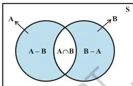
Special case — mutually exclusive: if \(A \cap B = \phi\), then \(P(A \cap B) = P(\phi) = 0\) and the formula becomes \(P(A \cup B) = P(A) + P(B)\), which is exactly axiom (iii).
Complement rule (NCERT, p. 302): since \(A\) and \(A’\) are mutually exclusive and together fill \(S\), \(P(A) + P(A’) = P(S) = 1\), so:
\[ P(A’) = 1 – P(A) \]
Three-event extension (Example 11, p. 309), needed in the Miscellaneous Exercise:
\[ P(A \cup B \cup C) = P(A) + P(B) + P(C) – P(A \cap B) – P(A \cap C) – P(B \cap C) + P(A \cap B \cap C) \]
The pattern: add the three singles, subtract the three pairwise overlaps, then add back the triple overlap — because the region \(A \cap B \cap C\) was subtracted too many times.
Worked Examples: Applying the Rules Step by Step
Three original problems, solved in the exact sequence the examiner expects. Work them on paper before reading the steps.
Example 1: Is this assignment valid? (Method: the two-condition test)
Step 1: Write the sample space and the assignment.
\(S = \{\omega_1, \omega_2, \omega_3, \omega_4, \omega_5\}\) with probabilities 0.1, 0.2, 0.15, 0.25, 0.3 in that order.
Step 2: Condition 1 — every value lies in [0, 1]: 0.1, 0.2, 0.15, 0.25, 0.3 all satisfy \(0 \leq P(\omega_i) \leq 1\).
Passed.
Step 3: Condition 2 — the sum: 0.1 + 0.2 + 0.15 + 0.25 + 0.3 = 1.00.
Passed.
Final answer: Valid, because both conditions hold.
Now two failing assignments on the same \(S\). Assignment X: 0.4, 0.1, -0.2, 0.3, 0.4 is invalid, because -0.2 is negative. Assignment Y: 0.5, 0.4, 0.3, 0.2, 0.7 is invalid, because the sum is 2.1, not 1.
Example 2: Two dice — P(sum is 7 or first die shows 4) (Method: addition theorem)
Step 1: Count the sample space.
Two distinct dice give ordered pairs, so \(n(S) = 6 \times 6 = 36\) outcomes.
- Step 1: Define \(A\) = ‘sum is 7’ and list it: \(A = \{(1,6), (2,5), (3,4), (4,3), (5,2), (6,1)\}\), so \(n(A) = 6\).
- Step 2: Define \(B\) = ‘first die shows 4’: \(B = \{(4,1), (4,2), (4,3), (4,4), (4,5), (4,6)\}\), so \(n(B) = 6\).
- Step 3: Find the overlap: \(A \cap B = \{(4,3)\}\), so \(n(A \cap B) = 1\).
- Step 4: Substitute into \(P(A \cup B) = P(A) + P(B) – P(A \cap B)\):
\[ P(A \cup B) = \frac{6}{36} + \frac{6}{36} – \frac{1}{36} = \frac{11}{36} \]
Final answer: \(P(A \cup B) = \frac{11}{36}\). The counts are in outcomes; the probability itself has no unit.
Example 3: Chips in a bowl — P(not blue) (Method: complement rule)
Step 1: Count the sample space.
The bowl holds 8 red, 5 green and 7 blue chips; one chip is drawn, so \(n(S) = 8 + 5 + 7 = 20\) outcomes.
- Step 1: \(P(\text{blue}) = \frac{7}{20}\), because 7 of the 20 chips are blue.
- Step 2: Use the complement rule \(P(\text{not blue}) = 1 – P(\text{blue})\):
\[ P(\text{not blue}) = 1 – \frac{7}{20} = \frac{13}{20} \]
Final answer: \(\frac{13}{20}\). Quick check: \(\frac{7}{20} + \frac{13}{20} = 1\), exactly as the complement rule requires.
Common Mistakes Students Make in Probability
The five slips below account for most lost marks in this chapter. Each row gives the error, the rule, and a way to verify your written answer.
| Mistake | Correct rule | How to check your answer |
|---|---|---|
| Writing \(P(A’) = P(A) – 1\) | \(P(A’) = 1 – P(A)\). Since \(A\) and \(A’\) are mutually exclusive and together fill \(S\), \(P(A) + P(A’) = 1\). | Add \(P(A)\) and \(P(A’)\); you must get exactly 1. |
| Adding \(P(A) + P(B)\) for any two events | Subtract the overlap: \(P(A \cup B) = P(A) + P(B) – P(A \cap B)\). | Ask: does any sample point lie in both \(A\) and \(B\)? If yes, you must subtract. |
| Counting two dice as 21 unordered pairs | Count 36 ordered pairs — the dice are distinct, so \((4,3)\) and \((3,4)\) are different outcomes. | Label the dice ‘first’ and ‘second’; list outcomes as ordered pairs \((x, y)\). |
| Accepting negative or greater-than-1 probabilities in an assignment | Reject the assignment; valid requires \(0 \leq P(\omega_i) \leq 1\) for all \(i\) and the sum equal to 1. | Run both conditions, not just the sum. |
| Treating ‘not mutually exclusive’ as identical to ‘not exhaustive’ | They are independent ideas: check \(A \cap B\) for mutually exclusive, \(A \cup B = S\) for exhaustive. | Test one at a time; a pair can be mutually exclusive and still not exhaustive. |
Exam Notes: What the Examiner Expects to See
Across the chapter’s exercises the same mark-earning pattern repeats. In a board-style probability question, this is the sequence the examiner looks for:
- Define the event in words first — ‘Let E be the event that …’.
- Write the sample space or state \(n(S)\) — for two dice, 36 is the total every later count is compared against.
- List the favourable set in braces — for sum questions, the listing itself carries marks.
- Write \(n(E)\) and \(n(S)\) separately, then form the fraction.
- Simplify to lowest terms — \(\frac{6}{36}\) must become \(\frac{1}{6}\).
For true/false questions such as Exercise 14.1 Q7, the reason earns the mark — quote one sample point to justify ‘not mutually exclusive’ (for example, 3 belongs to both ‘odd’ and ‘less than 4’).
For combination problems, give the denominator first (total ways), then the favourable count, then the fraction. For valid-assignment checks, show both conditions — the sum alone is not enough, as Assignment X in Example 1 shows.
Figure Walkthrough: Fig 14.1 and the Overlap Problem
The textbook’s Fig 14.1 is a standard two-circle Venn diagram. Read it in three parts:
- The rectangle is the whole sample space \(S\) — every possible outcome lives inside it.
- The two circles are events \(A\) and \(B\); the points inside a circle are exactly the outcomes of that event.
- The overlapping lens in the middle is \(A \cap B\), the outcomes belonging to both events.
When you compute \(P(A) + P(B)\), the lens is counted twice — once as part of \(A\), once as part of \(B\). Subtracting \(P(A \cap B)\) once fixes the double count, which is exactly what the addition theorem does.
When the circles do not overlap, \(A\) and \(B\) are mutually exclusive, the lens is empty, \(P(A \cap B) = P(\phi) = 0\), and the subtraction vanishes — the general formula becomes the axiom (iii) special case.
Where Probability Appears in Real Life
The chapter’s own examples are the best motivation — real settings, not invented ones:
- Entrance-test results (Example 7, pp. 304–305): two candidates with individual pass probabilities 0.05 and 0.10 and joint probability 0.02; the addition theorem and De Morgan’s law answer ‘both fail’, ‘at least one fails’ and ‘exactly one passes’. The axioms guarantee every computed probability stays inside [0, 1].
- Lotteries (Exercise 14.2 Q11, p. 307, and Miscellaneous Q4, p. 311): one winning combination out of all possible choices — the counting formula delivers the tiny probability, and the axioms confirm it is a valid number between 0 and 1.
- Committee selection (Example 8, p. 305): choosing 2 persons from 2 men and 2 women — the denominator \(\binom{4}{2}\) comes first, then the favourable counts. This is where Permutations and Combinations connects to probability.
Statistics looks at data that has already happened; probability predicts what happens next. The Class 11 Statistics notes cover the descriptive side of the same coin.
Probability Formulas: One-Table Revision
Every formula in the chapter, with its conditions, in one place (NCERT, pp. 299–302, 310, 313).
| Formula | Meaning of symbols | When to use |
|---|---|---|
| \(P(A) = \frac{n(A)}{n(S)}\) | n(A) = favourable outcomes, n(S) = total outcomes | Equally likely outcomes |
| \(P(A) = \sum P(\omega_i)\), \(\omega_i \in A\) | Sum of probabilities of the sample points in A | General, axiomatic approach |
| \(P(A \cup B) = P(A) + P(B) – P(A \cap B)\) | \(\cup\) = or, \(\cap\) = and | Any two events |
| \(P(A \cup B) = P(A) + P(B)\) | — | A and B mutually exclusive (\(A \cap B = \phi\)) |
| \(P(A’) = 1 – P(A)\) | \(A’\) = not A | Complement problems |
| \(P(A \cup B \cup C) = P(A) + P(B) + P(C) – P(A \cap B) – P(A \cap C) – P(B \cap C) + P(A \cap B \cap C)\) | Add singles, subtract pairs, add back the triple | Three events (Example 11, p. 309) |
| \(0 \leq P(\omega_i) \leq 1\) and \(\sum P(\omega_i) = 1\) | Sum over all outcomes of S | Checking whether an assignment is valid |
Revision Summary: Probability in One Page
- Event = subset of the sample space. Impossible = \(\phi\); sure = \(S\); simple = one sample point; compound = more than one.
- Algebra: not A = \(A’ = S – A\); A or B = \(A \cup B\); A and B = \(A \cap B\); A but not B = \(A – B\).
- Mutually exclusive means \(A \cap B = \phi\); exhaustive means the union is \(S\); both means pairwise disjoint AND union = \(S\).
- Three axioms: \(P(E) \geq 0\), \(P(S) = 1\), additive for disjoint events. Two validity checks: \(0 \leq P(\omega_i) \leq 1\) and all probabilities sum to 1.
- Equally likely outcomes: \(P(E) = \frac{n(E)}{n(S)}\).
- Addition theorem: \(P(A \cup B) = P(A) + P(B) – P(A \cap B)\).
- Complement: \(P(A’) = 1 – P(A)\).
Memory devices:
- Count twice, subtract once — the addition theorem. The overlap region was counted in both \(P(A)\) and \(P(B)\), so remove it exactly once.
- Total minus the part — the complement rule. All probabilities add to 1, so what is not A is 1 minus what is A.
Frequently Asked Questions
Why is P(not A) equal to 1 minus P(A) and not the other way around?
Because \(P(A) + P(A’) = 1\). The events \(A\) and \(A’\) are mutually exclusive and together fill \(S\), so their probabilities add to \(P(S) = 1\). Rearranging gives \(P(A’) = 1 – P(A)\), which is never negative because \(P(A)\) never exceeds 1.
Are mutually exclusive events always exhaustive?
No. Mutually exclusive requires \(A \cap B = \phi\); exhaustive requires the union to be \(S\). A pair can satisfy one without the other — ‘odd number’ and ‘even number’ on a die satisfy both, while ‘less than 4’ and ‘more than 5’ are mutually exclusive but their union \(\{1,2,3,6\}\) is not the whole of \(S\).
How do I check if a probability assignment is valid?
Test two conditions only: every assigned probability must lie between 0 and 1 inclusive, and the sum of all assigned probabilities must equal 1. If either condition fails, the assignment is invalid.
When can I add P(A) and P(B) without subtracting anything?
Only when A and B are mutually exclusive. Then \(A \cap B = \phi\), so \(P(A \cap B) = 0\), and the general formula \(P(A \cup B) = P(A) + P(B) – P(A \cap B)\) reduces to the simple sum. Otherwise the overlap is counted twice.
Why does a two dice experiment have 36 outcomes and not 21?
Because the two dice are distinct objects. The ordered pairs \((1,2)\) and \((2,1)\) are different outcomes, giving \(6 \times 6 = 36\) total outcomes. Counting 21 unordered pairs undercounts every pair with different numbers on the two dice.
What is the difference between simple and compound events?
A simple event has exactly one sample point, like \(\{HH\}\) in a two-coin toss. A compound event has more than one, like \(\{HT, TH\}\) meaning ‘exactly one tail’. A sample space with \(n\) elements has exactly \(n\) simple events.
Reference: NCERT Class 11 Mathematics textbook, chapter Probability.
Explore Class 11 Mathematics Notes
- Previous: Statistics
More for this chapter:
Class 11 Mathematics on LearnCBSE:
Related chapters:
- Sets notes
- Relations and Functions notes
- Trigonometric Functions notes