These limits and derivatives class 11 notes compress NCERT Chapter 12 into definitions students actually understand, every formula you need, fully worked examples with original numbers, and examiner-minded tips for last-minute revision. They are part of our broader Class 11 Mathematics notes, which sit inside the full Class 11 notes collection on this site.
Work top to bottom: first the derivative’s meaning (a rate of change), then the limit machinery it rests on, then the algebra rules for both. Each section carries the NCERT page number so you can jump back to the textbook where a point needs more depth.
The official NCERT PDF for Chapter 12 (kemh112.pdf) is free to download from ncert.nic.in if you want the full chapter alongside these notes.
The Intuitive Idea: Velocity as a Derivative
The chapter opens with a falling body. Drop a stone from a tall cliff and the distance it covers in \( t \) seconds is \( s = 4.9t^2 \) metres (NCERT, p. 218). The question: what is the velocity at the exact instant \( t = 2 \)?
Average velocity between two instants \( t_1 \) and \( t_2 \) is the distance travelled divided by the time interval: \( v = \frac{s(t_2)-s(t_1)}{t_2-t_1} \). For the first two seconds that gives \( \frac{19.6-0}{2-0} = 9.8 \) m/s (NCERT, p. 218).
The trick is to shrink the interval towards \( t = 2 \). Intervals ending at \( t = 2 \) give 14.7, 19.11, 19.355, 19.551 m/s as the start point creeps up to 1.99 s. Intervals starting at \( t = 2 \) give 20.09, 19.845, 19.649 m/s as the end point drops towards 2.01 s (NCERT, pp. 219–220).
Both sequences press towards one number near 19.6 m/s. That shared target is the instantaneous velocity at \( t = 2 \), and it is what we call the derivative of \( s = 4.9t^2 \) at \( t = 2 \) (NCERT, p. 220).
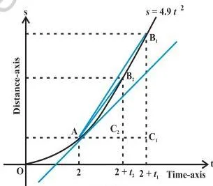
The image (Fig 12.1) translates the numbers into geometry on the \( s \)-\( t \) curve. Each ratio \( \frac{CB}{AC} \) is the slope of a chord; as the time interval collapses, the chords slide into the tangent at the point, so the instantaneous velocity equals the tangent’s slope (NCERT, p. 220).
Quick check with original numbers. A car’s position is \( s(t) = 6t^2 – 4t \) metres after \( t \) seconds. Average velocity from \( t=2 \) to \( t=2.1 \): \( \frac{s(2.1)-s(2)}{0.1} = \frac{18.06-16}{0.1} = 20.6 \) m/s. From \( t=2 \) to \( t=2.01 \): \( \frac{16.2006-16}{0.01} = 20.06 \) m/s. The values close in on 20 m/s, so the instantaneous velocity at \( t=2 \) is 20 m/s.
Real-life application — estimating speed from distance data. The same “known values, find the rate” pattern shows up when reservoir managers predict an overflow from water-depth readings, when rocket engineers compute the precise launch velocity of a satellite from its height over time, and when financial analysts track a stock’s swing from its present value (NCERT, p. 240).
Analysing how one quantity changes with another is also the core idea behind the statistics chapter notes.
Limits: Formal Definition and One-Sided Limits
A limit asks what value \( f(x) \) should take at \( x = a \), based purely on the values the function takes near \( a \). For \( h(x) = \frac{x^2-4}{x-2} \), \( x \neq 2 \), the function is undefined at 2, yet plugging in 1.99, 1.999, 2.001, 2.01 always lands near 4. We write \( \lim_{x \to 2} h(x) = 4 \) (NCERT, pp. 221–222).
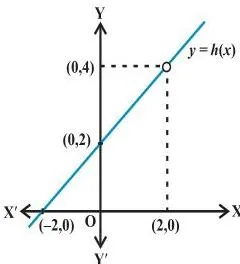
The graph above makes it visual: the line walks right up to a gap at \( x = 2 \), and the missing value would be 4. The limit is the value the function heads towards, whether or not the function actually reaches it there.
There are two directions from which \( x \) can approach \( a \): from the left (values smaller than \( a \)) or from the right (values larger than \( a \)). These give the left-hand limit \( \lim_{x \to a^-} f(x) \) and the right-hand limit \( \lim_{x \to a^+} f(x) \) (NCERT, p. 222).
| Quantity | What it means | Notation | When it exists |
|---|---|---|---|
| Left-hand limit | Expected value dictated by values of \( f \) to the left of \( a \) | \( \lim_{x \to a^-} f(x) \) | Values of \( f(x) \) settle on one number as \( x \to a^- \) |
| Right-hand limit | Expected value dictated by values of \( f \) to the right of \( a \) | \( \lim_{x \to a^+} f(x) \) | Values of \( f(x) \) settle on one number as \( x \to a^+ \) |
| Two-sided limit | The common expected value from both sides | \( \lim_{x \to a} f(x) \) | Only when LHL and RHL exist and are equal |
When one-sided limits disagree. Take \( f(x) = 1 \) for \( x \le 0 \) and \( f(x) = 2 \) for \( x \gt 0 \). The left-hand limit at 0 is 1, the right-hand limit is 2; because they differ, \( \lim_{x \to 0} f(x) \) does not exist — even though \( f(0) = 1 \) is perfectly defined (NCERT, p. 222).
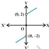
The jump graph above is Illustration 9 (NCERT, p. 227): \( f(x) = x-2 \) for \( x \lt 0 \), \( f(0) = 0 \), \( f(x) = x+2 \) for \( x \gt 0 \). Values from the left approach −2, values from the right approach +2, and no single limit exists.
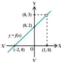
Illustration 10 (NCERT, p. 228) makes a second point: the value of a function and its limit at a point can be different. There \( f(1) = 0 \) but \( \lim_{x \to 1} f(x) = 3 \), because nearby behaviour — dictated by the branch \( x + 2 \) — is what a limit records.
Key Definitions: Limit, One-Sided Limits, Derivative
Quick-reference table for the central terms (definitions appear in NCERT, pp. 222 and 240).
| Term | Meaning | Example |
|---|---|---|
| Limit at a point | The value \( f(x) \) should assume at \( x = a \), dictated by values near \( a \) | \( \lim_{x \to 5}(x+10) = 15 \) |
| Left-hand limit | Expected value dictated by values of \( f \) to the left of \( a \) | \( \lim_{x \to 0^-} f(x) = 1 \) in the step function above |
| Right-hand limit | Expected value dictated by values of \( f \) to the right of \( a \) | \( \lim_{x \to 0^+} f(x) = 2 \) in the step function above |
| Derivative at a point | Rate of change of \( f \) as \( x \) changes through \( a \) | \( f'(a) = \lim_{h \to 0}\frac{f(a+h)-f(a)}{h} \); for \( f(x) = 3x \), \( f'(2) = 3 \) |
| Derivative function (first principle) | The function \( f'(x) \) defined wherever the defining limit exists | \( f'(x) = \lim_{h \to 0}\frac{f(x+h)-f(x)}{h} \); for \( f(x) = x^2 \), \( f'(x) = 2x \) |
Algebra of Limits: Rules for Sum, Product, Quotient
Theorem 1 (NCERT, p. 228): when both \( \lim_{x \to a} f(x) \) and \( \lim_{x \to a} g(x) \) exist, limits respect the four arithmetic operations.
- Sum: \( \lim_{x \to a}[f(x)+g(x)] = \lim_{x \to a} f(x) + \lim_{x \to a} g(x) \)
- Difference: \( \lim_{x \to a}[f(x)-g(x)] = \lim_{x \to a} f(x) – \lim_{x \to a} g(x) \)
- Product: \( \lim_{x \to a}[f(x)\cdot g(x)] = \left(\lim_{x \to a} f(x)\right)\left(\lim_{x \to a} g(x)\right) \)
- Quotient: \( \lim_{x \to a}\frac{f(x)}{g(x)} = \frac{\lim_{x \to a} f(x)}{\lim_{x \to a} g(x)} \), only when \( \lim_{x \to a} g(x) \neq 0 \)
Special case of the product rule: a constant factor pulls out, \( \lim_{x \to a}[\lambda f(x)] = \lambda \lim_{x \to a} f(x) \) (NCERT, p. 228).
Why the quotient needs a non-zero denominator limit. A quotient’s behaviour is only predictable when the denominator settles away from 0. If \( \lim g(x) = 0 \), the fraction can blow up, oscillate, or approach a finite number depending on how fast numerator and denominator each vanish — one rule cannot decide all those cases.
Method: Theorem 1 — split the sum and pull out constants.
Direct substitution would have worked too, since this is a polynomial.
- Step 1: Split the sum: \( \lim_{x \to 2}[4x^2 + 3x] = \lim_{x \to 2} 4x^2 + \lim_{x \to 2} 3x \).
- Step 2: Pull constants out and use \( \lim_{x \to 2} x = 2 \): \( 4(2^2) + 3(2) \).
\[ = 4(4) + 6 = 22 \]
Final answer: \( \lim_{x \to 2}(4x^2 + 3x) = 22 \), which equals \( f(2) \).
Limits of Polynomial and Rational Functions
Because \( \lim_{x \to a} x = a \), multiplying step by step gives \( \lim_{x \to a} x^n = a^n \). Adding the terms of a polynomial then yields the headline result: the limit of a polynomial at \( a \) is simply \( f(a) \) (NCERT, p. 229).
Theorem 2 (NCERT, p. 232): for a positive integer \( n \), \( \lim_{x \to a}\frac{x^n – a^n}{x-a} = na^{n-1} \). The remark extends the result to rational \( n \) when \( a \) is positive — this is what later lets you differentiate expressions like \( \sqrt{x} \) by hand.
For a rational function \( \frac{g(x)}{h(x)} \), first try substituting \( x = a \). If \( h(a) \neq 0 \), the limit is simply \( \frac{g(a)}{h(a)} \). Trouble starts when \( h(a) = 0 \):
- If \( g(a) \neq 0 \) — numerator stays non-zero while the denominator vanishes — the limit does not exist.
- If \( g(a) = 0 \) too — the \( \frac{0}{0} \) form — factor both polynomials, cancel the shared factor, then substitute (NCERT, pp. 229–231).
Method: factorisation for the \( \frac{0}{0} \) form.
Step 1: Substitute \( x = 3 \): numerator and denominator each give 0, so this is \( \frac{0}{0} \) — factorise.
\[ x^2 – 9 = (x-3)(x+3) \]
Step 2: Cancel \( (x-3) \).
This is allowed precisely because \( x \to 3 \) but \( x \neq 3 \).
\[ \lim_{x \to 3}\frac{(x-3)(x+3)}{x-3} = \lim_{x \to 3}(x+3),\quad x \neq 3 \]
Step 3: Substitute now: \( 3 + 3 = 6 \).
Final answer: \( \lim_{x \to 3}\frac{x^2-9}{x-3} = 6 \).
Example where the limit does not exist: \( \lim_{x \to 1}\frac{x+3}{(x-1)(x+2)} \). Substituting gives \( \frac{4}{0} \) — the numerator settles at 4 while the denominator collapses to 0, so the quotient has no finite limit.
Misconception autopsy — why substitution fails for \( \frac{0}{0} \). The form 0/0 is not a number, so the calculator-style answer “0/0 = 0” is meaningless. Two ratios that both look like 0/0 can genuinely approach different limits: \( \frac{x^2-4}{x-2} \to 4 \) while \( \frac{x-2}{x^2-4} \) has no finite limit at 2. Substitution cannot decide — you must identify the factor causing the vanishing and cancel it first.
Standard Trigonometric Limits and the Sandwich Theorem
Two structural theorems come first. Theorem 3: if \( f(x) \le g(x) \) and both limits exist, then \( \lim f(x) \le \lim g(x) \), so limits preserve order (NCERT, p. 234).
The Sandwich Theorem (Theorem 4) builds on this: if \( f(x) \le g(x) \le h(x) \) and \( \lim f(x) = \lim h(x) = l \), then \( \lim g(x) = l \) (NCERT, p. 234).
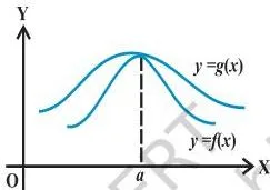
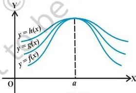
The two graphs above show the intuition: a function trapped between two others that meet at a common limit is forced to that same limit.
The key inequality (NCERT, p. 235): \( \cos x \lt \frac{\sin x}{x} \lt 1 \) for \( 0 \lt |x| \lt \frac{\pi}{2} \). Its geometric proof compares areas in the unit circle: triangle \( OAC \) is smaller than sector \( OAC \), which is smaller than triangle \( OAB \). That yields \( OA\sin x \lt OA\cdot x \lt OA\tan x \), i.e.
\( \sin x \lt x \lt \tan x \); dividing by \( \sin x \) (positive here) and taking reciprocals gives the inequality.
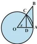
Since \( \cos x \to 1 \) as \( x \to 0 \), the Sandwich Theorem squeezes \( \frac{\sin x}{x} \) down to 1 (NCERT, p. 235). The companion limit follows from \( 1 – \cos x = 2\sin^2\left(\frac{x}{2}\right) \): \( \frac{1-\cos x}{x} = \frac{\sin(x/2)}{x/2}\cdot\sin(x/2) \to 1\cdot 0 = 0 \) (NCERT, p. 236).
\[ \lim_{x \to 0}\frac{\sin x}{x} = 1,\qquad \lim_{x \to 0}\frac{1-\cos x}{x} = 0 \]
Memory device: “Match the sine to the floor.” For \( \frac{\sin x}{x} \to 1 \), the argument inside sine and the denominator must be the same quantity heading to 0. That is why \( \frac{\sin(7x)}{7x} \to 1 \) but \( \frac{\sin x}{x^2} \) does not.
Whenever you rescale, write the argument and the denominator identically (both \( 5x \), both \( 3x \)) before applying the standard limit.
Method: rewrite each piece in the “sine over identical argument” shape, then use \( \frac{\sin t}{t} \to 1 \).
\[ \frac{\sin 5x}{\sin 3x} = \frac{\sin 5x}{5x}\cdot\frac{5x}{3x}\cdot\frac{3x}{\sin 3x} = \frac{5}{3}\cdot\frac{\sin 5x}{5x}\cdot\frac{1}{\frac{\sin 3x}{3x}} \]
Step: as \( x \to 0 \), both \( 5x \) and \( 3x \) tend to 0, so each standard limit equals 1:
\[ \lim_{x \to 0}\frac{\sin 5x}{\sin 3x} = \frac{5}{3}\cdot 1 \cdot \frac{1}{1} = \frac{5}{3} \]
Final answer: \( \frac{5}{3} \). Angle arguments are in radians throughout.
The trigonometric limit work in this section draws on the identities covered in the trigonometric functions notes.
Derivatives: Definition and First Principle
Definition 1 (NCERT, p. 240): the derivative of \( f \) at a point \( a \) is \( f'(a) = \lim_{h \to 0}\frac{f(a+h)-f(a)}{h} \), provided this limit exists. It quantifies how \( f \) changes at \( a \) as \( x \) changes.
Definition 2 / first principle (NCERT, p. 242): the derivative function \( f'(x) = \lim_{h \to 0}\frac{f(x+h)-f(x)}{h} \), defined wherever the limit exists. Common notations are \( f'(x) \), \( \frac{dy}{dx} \), and \( Df(x) \) — all name the same rate of change.
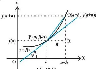
The image carries the geometric meaning: \( \frac{f(a+h)-f(a)}{h} \) is the slope of the chord \( PQ \). As \( h \to 0 \), Q slides into P and the chord becomes the tangent, so the derivative is the slope of the tangent at that point — \( f'(a) = \tan\psi \) (NCERT, p. 242).
This tangent-slope idea connects to the coordinate geometry you meet in the three-dimensional geometry notes.
Method: first principle — substitute, expand, cancel \( h \), then take the limit.
- Step 1: Write the definition at \( a = 2 \): \( f'(2) = \lim_{h \to 0}\frac{f(2+h)-f(2)}{h} \).
- Step 2: \( f(2+h) = 5(2+h)^2 – 2(2+h) + 1 = 5(4+4h+h^2) – 4 – 2h + 1 = 17 + 18h + 5h^2 \), and \( f(2) = 20 – 4 + 1 = 17 \).
- Step 3: Form the difference quotient: \( \frac{(17+18h+5h^2)-17}{h} = 18 + 5h \).
- Step 4: Let \( h \to 0 \): \( 18 + 5(0) = 18 \).
Final answer: \( f'(2) = 18 \).
Algebra of Derivatives: Product and Quotient Rules
Theorem 5 (NCERT, p. 244): when derivatives exist in a common domain, the following rules hold.
- Sum: \( \frac{d}{dx}[f+g] = \frac{df}{dx} + \frac{dg}{dx} \)
- Difference: \( \frac{d}{dx}[f-g] = \frac{df}{dx} – \frac{dg}{dx} \)
- Product rule: \( \frac{d}{dx}[fg] = \frac{df}{dx}\cdot g + f\cdot\frac{dg}{dx} \)
- Quotient rule: \( \frac{d}{dx}\left(\frac{f}{g}\right) = \frac{\frac{df}{dx}\cdot g – f\cdot\frac{dg}{dx}}{g^2} \), needing \( g \neq 0 \)
With \( u = f(x) \) and \( v = g(x) \), these become the Leibnitz rules (NCERT, p. 245): \( (uv)’ = u’v + uv’ \) and \( \left(\frac{u}{v}\right)’ = \frac{u’v – uv’}{v^2} \).
Why the product rule is not “differentiate each factor”. When both factors vary, the total change of the product gets a contribution from \( u \) changing while \( v \) stays, plus a contribution from \( v \) changing while \( u \) stays. Those two strips of growth are \( u’v + uv’ \).
The wrong guess \( u’v’ \) only counts the tiny corner where both change at once, missing the two main contributions.
Product rule example — \( f(x) = (3x+2)(x^2-1) \).
\[ f'(x) = 3(x^2-1) + (3x+2)(2x) \]
\[ = 3x^2 – 3 + 6x^2 + 4x = 9x^2 + 4x – 3 \]
Final answer: \( f'(x) = 9x^2 + 4x – 3 \).
Quotient rule example — \( f(x) = \frac{x+1}{x-2} \) (valid for \( x \neq 2 \)).
\[ f'(x) = \frac{1\cdot(x-2) – (x+1)\cdot 1}{(x-2)^2} = \frac{x-2-x-1}{(x-2)^2} \]
\[ = -\frac{3}{(x-2)^2} \]
Final answer: \( f'(x) = -\frac{3}{(x-2)^2} \) for all \( x \neq 2 \).
Derivatives of Standard Functions
Each derivative below is proved from the first principle together with the standard trigonometric limits (NCERT, pp. 245–247).
| Function | Derivative |
|---|---|
| \( x^n \) | \( nx^{n-1} \) |
| \( \sin x \) | \( \cos x \) |
| \( \cos x \) | \( -\sin x \) |
| \( \tan x \) | \( \sec^2 x \) |
| \( \cot x \) | \( -\cosec^2 x \) |
| \( \sec x \) | \( \sec x \tan x \) |
| \( \cosec x \) | \( -\cosec x \cot x \) |
For example, \( \frac{d}{dx}\sin x = \lim_{h \to 0}\frac{\sin(x+h)-\sin x}{h} = \cos x \cdot 1 \), using \( \sin A – \sin B = 2\cos\frac{A+B}{2}\sin\frac{A-B}{2} \) and \( \frac{\sin(h/2)}{h/2} \to 1 \) (NCERT, p. 247).
Method: write \( \tan x = \frac{\sin x}{\cos x} \) and apply the quotient rule.
\[ \frac{d}{dx}\tan x = \frac{(\cos x)(\cos x) – (\sin x)(-\sin x)}{\cos^2 x} = \frac{\cos^2 x + \sin^2 x}{\cos^2 x} \]
\[ = \frac{1}{\cos^2 x} = \sec^2 x \]
Final answer: \( \frac{d}{dx}\tan x = \sec^2 x \).
Limits and Derivatives Class 11 Notes: Master Formula Sheet
One compact grid of everything from the chapter (formulas appear across NCERT, pp. 228, 232, 235–236, 244–245, 247).
| Type | Formula | Conditions |
|---|---|---|
| Sum of limits | \( \lim[f+g] = \lim f + \lim g \) | Both limits exist |
| Product of limits | \( \lim[f\cdot g] = (\lim f)(\lim g) \) | Both limits exist |
| Quotient of limits | \( \lim\frac{f}{g} = \frac{\lim f}{\lim g} \) | Both exist and \( \lim g \neq 0 \) |
| Constant multiple | \( \lim \lambda f = \lambda \lim f \) | — |
| Power limit | \( \lim_{x \to a} x^n = a^n \) | Polynomial limit equals \( f(a) \) |
| Standard limit 1 | \( \lim_{x \to a}\frac{x^n-a^n}{x-a} = na^{n-1} \) | \( n \) positive integer (rational \( n \), \( a \gt 0 \)) |
| Standard limit 2 | \( \lim_{x \to 0}\frac{\sin x}{x} = 1 \) | \( x \) in radians |
| Standard limit 3 | \( \lim_{x \to 0}\frac{1-\cos x}{x} = 0 \) | \( x \) in radians |
| Derivative at a point | \( f'(a) = \lim_{h \to 0}\frac{f(a+h)-f(a)}{h} \) | Limit exists |
| Derivative function | \( f'(x) = \lim_{h \to 0}\frac{f(x+h)-f(x)}{h} \) | First principle |
| Sum / difference | \( (u \pm v)’ = u’ \pm v’ \) | Derivatives defined in common domain |
| Product (Leibnitz) | \( (uv)’ = u’v + uv’ \) | — |
| Quotient | \( \left(\frac{u}{v}\right)’ = \frac{u’v-uv’}{v^2} \) | \( v \neq 0 \) |
| Power derivative | \( \frac{d}{dx}x^n = nx^{n-1} \) | Proved for positive integers in this course |
| Trig derivatives | \( \frac{d}{dx}\sin x = \cos x \), \( \frac{d}{dx}\cos x = -\sin x \), \( \frac{d}{dx}\tan x = \sec^2 x \) | — |
Worked Examples: Limits and Derivatives
Example A — limit of a rational function by factorisation: \( \lim_{x \to 4}\frac{x^2-16}{x-4} \).
Step 1: Substitute \( x=4 \): \( \frac{16-16}{4-4} = \frac{0}{0} \), so factorise the numerator.
\[ x^2 – 16 = (x-4)(x+4) \]
Step 2: Cancel \( (x-4) \) — allowed because \( x \to 4 \) but \( x \neq 4 \).
\[ \lim_{x \to 4}\frac{(x-4)(x+4)}{x-4} = \lim_{x \to 4}(x+4) \]
Step 3: Substitute: \( 4 + 4 = 8 \).
Final answer: \( \lim_{x \to 4}\frac{x^2-16}{x-4} = 8 \).
Example B — trigonometric limit: \( \lim_{x \to 0}\frac{1-\cos 2x}{x^2} \).
Step 1: Substitution gives \( \frac{0}{0} \).
Apply the identity \( 1 – \cos 2x = 2\sin^2 x \).
\[ \frac{1-\cos 2x}{x^2} = \frac{2\sin^2 x}{x^2} = 2\left(\frac{\sin x}{x}\right)^2 \]
Step 2: Use the standard limit \( \frac{\sin x}{x} \to 1 \).
\[ \lim_{x \to 0}\frac{1-\cos 2x}{x^2} = 2(1)^2 = 2 \]
Final answer: \( 2 \).
Example C — derivative from first principle: \( f(x) = 2x^3 – 3x \), find \( f'(1) \).
- Step 1: \( f'(x) = \lim_{h \to 0}\frac{f(x+h)-f(x)}{h} \).
- Step 2: \( f(x+h) = 2(x+h)^3 – 3(x+h) = 2x^3 + 6x^2h + 6xh^2 + 2h^3 – 3x – 3h \).
Subtract \( f(x) = 2x^3 – 3x \): the difference is \( 6x^2h + 6xh^2 + 2h^3 – 3h \).
- Step 1: Divide by \( h \): \( 6x^2 + 6xh + 2h^2 – 3 \).
- Step 2: Let \( h \to 0 \): \( f'(x) = 6x^2 – 3 \).
At \( x = 1 \), \( f'(1) = 6 – 3 = 3 \).
Final answer: \( f'(1) = 3 \).
Common Mistakes to Avoid
Five chapter-specific errors cost marks every year. The table pairs each error with the correct rule and a quick self-check.
| Mistake | Correct rule | How to check your answer |
|---|---|---|
| Substituting directly when the limit is \( \frac{0}{0} \) | Factorise, cancel the common factor, then substitute | Plug in nearby numbers (1.99, 2.01) — both must hug the same value |
| Declaring a limit exists without checking both sides | Check LHL and RHL; both must exist and agree | If the graph jumps or the two sides disagree, the limit does not exist |
| Applying \( \frac{\sin x}{x} \to 1 \) to any argument | Use it only as \( x \to 0 \), in radians, with identical argument and denominator | Rewrite as \( \frac{\sin(kx)}{kx} \) and confirm \( kx \to 0 \) |
| Using the product rule as \( (uv)’ = u’v’ \) | Use the Leibnitz rule \( (uv)’ = u’v + uv’ \) | Differentiate keeping one factor, then the other, and add |
| Cancelling \( (x-a) \) as if \( x \) could equal \( a \) | Cancel only because \( x \to a \) while \( x \neq a \) | Write “as \( x \neq a \)” after every cancellation inside a limit |
Spotlight on the cancellation error. Students write \( \lim_{x \to 2}\frac{x^2-4}{x-2} = \frac{(x-2)(x+2)}{(x-2)} = x+2 \) and then treat \( x+2 \) as if it were the original function everywhere. The correction: \( \frac{x^2-4}{x-2} \) is not defined at \( x = 2 \). Only after cancelling — valid precisely because \( x \neq 2 \) in the limiting process — do we reach \( x+2 \), whose limit is \( 4 \).
So the limit equals 4, but \( f(2) \) does not even exist.
Exam Notes: What CBSE Looks For
- Rational-function limits: substitute first, then factorise for the \( \frac{0}{0} \) cases (pattern of Exercise 12.1, Q2–Q8).
- Trigonometric limits: the two standard limits, with angles in radians (Exercise 12.1, Q13–Q21).
- One-sided limits and piecewise functions decide whether a limit exists (Exercise 12.1, Q23–Q30).
- First-principle derivatives for simple polynomials and trigonometric functions (Exercise 12.2, Q4 and Q10; Miscellaneous Q1, Q14).
- Method marks matter: writing the correct setup — the quotient rule formula, the standard-limit shape — earns marks even if the final simplification slips.
- Write “as \( x \neq a \)” next to each cancellation inside a limit; it shows you understand the limiting condition.
For quick reference back to the full curriculum, the CBSE notes index lists every chapter page on this site.
Revision Summary: One-Page Recap
A recall aid: concept, the rule in one line, and where the textbook proves it.
| Concept | Definition / Rule | Key Formula | Textbook page |
|---|---|---|---|
| Limit | Common expected value; exists when LHL = RHL | \( \lim_{x \to a} f(x) \) | p. 222 |
| One-sided limits | Expected value from the left / from the right | \( \lim_{x \to a^-} f(x) \), \( \lim_{x \to a^+} f(x) \) | p. 222 |
| Algebra of limits | Limits pass through \( + \), \( – \), \( \times \), \( \div \) (division needs non-zero denominator) | Theorem 1 | p. 228 |
| Polynomial limits | Limit equals \( f(a) \) | \( \lim_{x \to a} x^n = a^n \) | p. 229 |
| Standard limits | Three limits you quote directly | \( \frac{x^n-a^n}{x-a} \to na^{n-1} \); \( \frac{\sin x}{x} \to 1 \); \( \frac{1-\cos x}{x} \to 0 \) | pp. 232, 235–236 |
| Derivative definition | Rate of change of \( f \) at a point | \( f'(a) = \lim_{h \to 0}\frac{f(a+h)-f(a)}{h} \) | p. 240 |
| Derivative rules | Sum, product, quotient | \( (uv)’ = u’v + uv’ \); \( \left(\frac{u}{v}\right)’ = \frac{u’v-uv’}{v^2} \) | pp. 244–245 |
| Standard derivatives | Power and trigonometric derivatives | \( \frac{d}{dx}x^n = nx^{n-1} \); \( \frac{d}{dx}\sin x = \cos x \), etc. | pp. 245, 247 |
Frequently Asked Questions
Why is the limit of \( \frac{\sin x}{x} \) equal to 1, and how do I use it?
The Sandwich Theorem forces it. For \( 0 \lt |x| \lt \frac{\pi}{2} \), the unit-circle area comparison gives \( \cos x \lt \frac{\sin x}{x} \lt 1 \). Since \( \cos x \to 1 \) as \( x \to 0 \), the squeezed function must also approach 1. To use it, the angle inside sine must equal the denominator and both must tend to 0 (all in radians), e.g.
\( \frac{\sin 7x}{7x} \to 1 \).
How do I find a limit when direct substitution gives 0/0?
Do not stop — factor the numerator and denominator, cancel the common factor (valid because \( x \neq a \) in the limit), and substitute again. For trigonometric forms, rewrite with the standard limits, like turning \( \frac{1-\cos x}{x} \) into \( \frac{\sin(x/2)}{x/2}\cdot\sin(x/2) \).
What is the difference between the derivative at a point and the derivative function?
The derivative at a point \( f'(a) = \lim_{h \to 0}\frac{f(a+h)-f(a)}{h} \) is a single number: the rate of change at that one spot.
The derivative function \( f'(x) = \lim_{h \to 0}\frac{f(x+h)-f(x)}{h} \) is defined wherever that limit exists and assigns a slope to every point in its domain at once.
When should I use the product rule versus the quotient rule?
Use the product rule when the function is one expression times another, \( uv \) — for example \( (3x+2)(x^2-1) \). Use the quotient rule when one expression is divided by another, \( \frac{u}{v} \), requiring \( v \neq 0 \). The quotient rule is the product rule’s close cousin: \( \frac{u’v – uv’}{v^2} \), with a minus sign and the square of the denominator.
How do I apply the first principle to find the derivative of a function?
Start from \( f'(x) = \lim_{h \to 0}\frac{f(x+h)-f(x)}{h} \). Substitute \( x+h \) into the function, subtract \( f(x) \), simplify and divide through by \( h \), then let \( h \to 0 \). With \( f(x) = 2x^3 – 3x \), expanding \( (x+h)^3 \) and cancelling \( h \) leaves \( 6x^2 + 6xh + 2h^2 – 3 \), whose limit is \( 6x^2 – 3 \).
Reference: NCERT Class 11 Mathematics textbook, chapter Limits and Derivatives.
Explore Class 11 Mathematics Notes
- Previous: Introduction to Three Dimensional Geometry
- Next: Statistics
More for this chapter:
Class 11 Mathematics on LearnCBSE:
Related chapters:
- Sets notes
- Relations and Functions notes
- Trigonometric Functions notes