
These revision notes condense Chapter 3, Organisation of Data, from the NCERT Class 11 Statistics for Economics textbook into one page you can revise from quickly.
Everything essential is here: what raw data is and why it must be ordered, the four types of classification, continuous and discrete variables, the anatomy of a frequency distribution (class limits, class interval, class mark), inclusive and exclusive classes, tally marking, and the special cases that follow.
These notes follow the 2026-27 session, and every key idea carries an NCERT page reference so you can cross-check any point in the textbook.
The page is built like a revision session: definitions and rules first, then three fully worked examples on fresh numbers, then the common-mistakes table and guidance on writing complete answers. If you have only a few minutes, jump to the five-minute recap at the end.
You can also verify any table or figure against the official NCERT PDF of Chapter 3, Organisation of Data, on ncert.nic.in.
This page is part of the Class 11 Economics notes series on this site; browse the whole set from that hub, or find every subject from the main CBSE notes library.
Chapter at a glance: from raw data to frequency distribution
Organisation of Data builds in one direction: raw data first, then classification, then a frequency distribution. Each stage answers a specific question, and the next stage cannot start until the previous one is finished (NCERT, pp. 23–36).
| Stage | Question it answers | Outcome |
|---|---|---|
| 1. Raw data | What did we collect, exactly as collected? | Unordered observations, e.g. Tables 3.1 and 3.2 (p. 24) |
| 2. Classification | On what basis do we group? | Chronological, spatial, qualitative or quantitative classes (pp. 25–27) |
| 3. Variable check | Is the variable continuous or discrete? | Decides grouped classes vs a frequency array (p. 28) |
| 4. Class formation | How many classes, of what size, with what limits? | A frequency distribution with class marks (pp. 29–30) |
| 5. Frequency count | How many observations in each class? | Tally marks → class frequencies (p. 32) |
| 6. Special cases | Are classes continuous? Is grouping losing detail? | Continuity adjustment, unequal classes, frequency array, bivariate distribution (pp. 31–36) |
Study targets — the chapter’s stated objectives (p. 22) double as a test of your revision. By the end you should be able to:
- classify raw data for further statistical analysis;
- distinguish quantitative from qualitative classification;
- prepare a frequency distribution table;
- apply the technique of forming classes;
- use the method of tally marking; and
- differentiate univariate from bivariate frequency distributions.
If the ground-level ideas of the course feel shaky, see the Class 11 notes collection for the full set of subjects in this class.
Raw data: why order matters before analysis
Raw data is data exactly as it was collected — unclassified, unordered observations. NCERT opens the chapter with your local kabadiwallah: he ties newspapers together, sacks the glass bottles, heaps the metals, and sorts them into “iron”, “copper”, “aluminium”, “brass”. Without that sorting, finding one requested item in a growing pile of junk becomes impossible (NCERT, pp. 23–24).
Data behaves the same way.
The chapter’s two raw tables show the problem. Table 3.1 lists marks in mathematics of 100 students in no particular order; Table 3.2 lists the monthly household food expenditure (in rupees) of 50 households, also unordered (p. 24).
- The ordering problem: to find the highest mark in Table 3.1 you must first sort all 100 marks in ascending or descending order — a tedious task that grows with every extra record (p. 24).
- The summarising problem: from Table 3.2 you cannot see the average monthly food expenditure of the 50 households without first arranging the values (p. 24).
- The scale problem: the Census of India contacted about 20 crore persons in Census 2001. Raw census data is so large and fragmented that reading it directly is almost impossible; once classified by gender, education, marital status and occupation, the structure of India’s population becomes understandable (p. 25).
The purpose of classification, therefore, is to bring order to the data so it can be subjected to statistical analysis easily (p. 22). Raw data consists of observations on variables, and how you classify depends on the purpose you have in mind (p. 25).
The four ways to classify data
Classification is arranging or organising things into groups or classes based on some criteria (NCERT, p. 23). The same data can be grouped in four ways, depending on the purpose.
| Type of classification | Basis of grouping | Chapter example | Page |
|---|---|---|---|
| Chronological | Time — years, quarters, months, weeks | Population of India by census years, 1951–2011 | p. 25 |
| Spatial | Geographical location — country, state, city | Yield of wheat (kg/hectare) by country, NCERT table (p. 26) | p. 26 |
| Qualitative | Attributes (gender, literacy, religion, marital status) that cannot be measured | Population grouped first by gender, then by marital status | p. 26 |
| Quantitative | Measurable characteristics such as height, weight, age, income, marks | Marks of 100 students grouped into classes of 10 | p. 27 |
Three details help you identify the type from any given table:
- Time series: when chronological classification is by years, the variable involved is called a time series — the population series in Example 1 is one (p. 25).
- Stages of qualitative classification: qualitative data can be classified in stages. NCERT’s Example 3 first splits the population into male and female (presence or absence of the attribute “male”), then subdivides each group into married and unmarried (p. 26).
- Quantitative outcome: Example 4 turns the raw marks of 100 students into ten classes, 0–10 up to 90–100 — a quantitative classification (p. 27).
Continuous vs discrete variables: know this before grouping
A variable is a characteristic that takes different values. Which summary you build depends on which kind of variable you are handling (NCERT, pp. 27–28).
- Continuous variable: can take any numerical value — whole numbers, fractions, and values that are not exact fractions such as \(\sqrt{2} = 1.414\). Height, weight, time and distance are continuous. A student growing from 90 cm to 150 cm passes through every value in between, including 90.85 cm and 149.99 cm (p. 27).
- Discrete variable: changes in finite jumps and skips the intermediate values. The number of students in a class can be 25 or 26 but never 25.5 — “half a student” is absurd (p. 28).
The edge case that traps students: a discrete variable can still take fractional values. If X takes values 1/8, 1/16, 1/32, …, it is still discrete, because there is no value between adjacent terms — it jumps from 1/8 to 1/16 and cannot take anything in between (p. 28).
| Feature | Continuous variable | Discrete variable |
|---|---|---|
| Values it can take | Any numerical value in a range | Only certain values, with nothing between adjacent ones |
| How it changes | Smoothly, in infinite gradations | In finite jumps |
| Fractions possible? | Yes | Only when no value lies between adjacent values (e.g. 1/8, 1/16) |
| Examples | Height, weight, time, distance | Number of students, size of a household |
| Consequence for grouping | Grouped into class intervals | Frequency array (one frequency per value) |
Why this matters: this single distinction decides what your final table looks like. Continuous data is grouped into classes (a frequency distribution); discrete data can be shown as a frequency array where each integral value keeps its own frequency (p. 35). Variables were introduced at the start of the book — the Why Economics notes give that foundation if you need it.
Frequency distribution essentials: classes, limits, interval and class mark
A frequency distribution is a comprehensive way to classify raw data of a quantitative variable: it shows how different values of the variable are distributed across classes, together with their class frequencies (NCERT, p. 28). The marks data of 100 students, for example, is grouped into ten classes from 0–10 to 90–100.
Class frequency is the number of values inside a particular class. In the NCERT marks table the class 30–40 contains seven marks — 30, 37, 34, 30, 35, 39 and 32 — so its class frequency is 7 (p. 28).
- Class limits: the two ends of a class. The class 60–70 has lower class limit 60 and upper class limit 70 (p. 28).
- Class interval (class width): the difference between the upper and lower class limits. For 60–70 it is \(70 – 60 = 10\) (p. 28).
- Class mark (mid-point): the middle value of the class, \(\frac{\text{upper limit} + \text{lower limit}}{2}\). For 60–70 it is \(\frac{70 + 60}{2} = 65\) (p. 29).
The excerpt below from NCERT’s Table 3.3 shows the pattern for three classes (p. 29):
| Class | Frequency | Lower class limit | Upper class limit | Class mark |
|---|---|---|---|---|
| 10–20 | 8 | 10 | 20 | 15 |
| 30–40 | 7 | 30 | 40 | 35 |
| 60–70 | 19 | 60 | 70 | 65 |
The rule that drives everything later: once raw data is grouped, individual observations are no longer used in calculations — each class is represented by its class mark (p. 29).
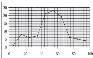
Fig 3.1 is the frequency curve of the 100-students marks distribution (p. 29). A frequency curve is a graphic representation of a frequency distribution, and it is drawn by plotting class marks on the X-axis and frequencies on the Y-axis.
This is the first payoff of class marks: without them there would be nothing to plot, because the raw values inside a class have already been merged into one representative number.
Inclusive and exclusive class intervals: where does the boundary value go?
Class intervals come in two forms, and the difference is exactly one question: is a value equal to a class limit counted in the class, or not? (NCERT, p. 30) Inclusive class intervals include both limits in the class: 0–10, 11–20, 21–30, … Here the value 10 belongs to the class 0–10.
Exclusive class intervals exclude one limit: 0–10, 10–20, 20–30, … The convention must be fixed in advance — either the upper limit is excluded (so 10 belongs to 10–20) or the lower limit is excluded (so 10 belongs to 0–10) (p. 31).
The NCERT marks table uses upper limit excluded. In this convention a class like 30–40 is read as “30 and above, but under 40” — the same way NCERT reads the classes in its weight example: “30 Kg and above and under 40 Kg” (p. 31).
| Feature | Inclusive classes | Exclusive classes |
|---|---|---|
| Form | 0–10, 11–20, 21–30 | 0–10, 10–20, 20–30 |
| Both limits included? | Yes | No — one limit is excluded |
| Value on a boundary (e.g. 10) | Stays in its own class (0–10) | Goes to the next class if the upper limit is excluded (10–20) |
| Gap between successive classes? | Yes (10 followed by 11) | No — classes are continuous |
| Typical use | Often used for continuous variables, then adjusted | Clean for continuous data without gaps |
| Suited to discrete variables? | Yes | Yes — either form works for a discrete variable (p. 30) |
The 40 puzzle, solved. NCERT, p. 28 asks why 40 — which appears twice in the raw marks — is not counted in the class 30–40. The answer is the exclusive method: the upper limit of a class is excluded and belongs to the next class, so both 40s are tallied into the class 40–50.
If they had been counted in 30–40, that class’s frequency would have been 9 instead of 7. NCERT confirms the rule in its tally discussion: “If someone obtains 40 marks, a tally is put against the class 40–50” (pp. 32–33).
Making inclusive classes continuous: the adjustment rule
When inclusive classes are used for a continuous variable, a gap appears between successive classes. In NCERT’s income table of 550 employees (Table 3.4), the first class ends at 899 and the next begins at 900 — a gap of 1, which breaks the continuity of the “income” variable (NCERT, pp. 31–32). The adjustment rule removes the gap in four steps:
- Find the difference between the lower limit of the second class and the upper limit of the first class: \(900 – 899 = 1\).
- Divide the difference by 2: \(1 \div 2 = 0.5\).
- Subtract this half from the lower limit of every class.
- Add this half to the upper limit of every class.
Applying the rule to the income data turns 800–899 into 799.5–899.5, 900–999 into 899.5–999.5, and so on (Table 3.5, p. 32). A fresh mini-example: classes 100–199 and 200–299 have gap \(200 – 199 = 1\), half-gap 0.5, and become 99.5–199.5 and 199.5–299.5.
The adjusted class mark is then computed on the adjusted limits:
\[ \text{Adjusted class mark} = \frac{\text{Adjusted upper limit} + \text{Adjusted lower limit}}{2} \]
The midpoint is unchanged by the adjustment: the 0.5 subtracted from the lower limit and the 0.5 added to the upper limit cancel out exactly, so the adjusted class mark equals the class mark you would have calculated before adjustment.
The five decisions behind every frequency distribution
NCERT, p. 29 lists five questions you must settle before building any frequency distribution. They form a practical checklist.
| Decision | Standard answer | Why it is made this way |
|---|---|---|
| 1. Equal or unequal class intervals? | Equal, as the default | Unequal only when the range is very high (like income, from near zero to hundreds of crores) or when many values cluster in a small part of the range; equal intervals then create too many classes or suppress information at the extremes (pp. 29–30) |
| 2. How many classes? | Usually between 6 and 15 | Too few hides the shape of the data; too many brings back the mess of raw data (p. 30) |
| 3. What class size? | Tied to the range and the chosen number of classes | Size and number are interlinked: fix one and the other follows — with a range of 100 and 10 classes, each class is automatically 10 wide (p. 30) |
| 4. What class limits? | Definite and clearly stated; avoid open-ended classes like “70 and over” | Limits should make the frequencies of each class concentrate near the middle of the class (p. 30) |
| 5. How to find the frequencies? | By tally marks against each class | Tallying in groups of five keeps counting fast and accurate (pp. 32–33) |
Two formulas wrap decisions 2 and 3 together:
\[ \text{Range} = \text{Largest value} – \text{Smallest value} \]
\[ \text{Number of classes} = \frac{\text{Range}}{\text{Size of class interval}} \]
For the marks example: the values run from 0 to 100, so the range is 100, and with ten classes the interval is automatically 10 (p. 30). Work the two formulas in the same breath — changing the class size automatically changes the number of classes.
Tally marking: counting observations accurately
Before any table, one definition: the frequency of an observation is how many times that observation occurs in the raw data. In Table 3.1 the value 40 occurs three times and 49 occurs five times, so their frequencies are 3 and 5 (NCERT, p. 32).
For classes, you never count directly — you tally:
- Put one stroke (/) against a class for each observation that falls in it.
- Four strokes are written as ////, and the fifth stroke is placed across them, making a bundle of five.
- Count bundles of five first, then add the remaining singles. Sixteen tallies are written as //// //// //// / (p. 33).
- The class frequency equals the number of tallies against that class (p. 33).
NCERT’s Table 3.6 shows the complete tally marking for the 100 mathematics marks, with columns Class | Observations | Tally Mark | Frequency | Class Mark (pp. 32–33) — it is the model for any tally table you build. You will construct one with fresh data in Worked example 1 below.
Loss of information and when unequal classes work better
Grouping raw data has a built-in shortcoming: it summarises, and a summary drops detail. This is called loss of information (NCERT, pp. 33–34).
Take the NCERT class 20–30, which holds six actual marks: 25, 25, 20, 22, 25 and 28. Once grouped, the class shows only its frequency (6) — the six values vanish, and all of them are treated as equal to the class mark 25. Every later statistical calculation then uses class marks, not the original observations (p. 34).
That is the trade-off: you gain a comprehensible table, but you lose the identity of each observation.
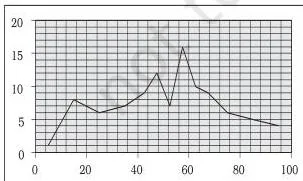
Fig 3.2 is the frequency curve of the unequal-class distribution in Table 3.7 (p. 35). The plotting rule is unchanged — class marks on the X-axis, frequencies on the Y-axis — so compare it with Fig 3.1: the two curves differ because the classes behind them differ, not because the method changed. NCERT’s activity on p. 35 asks you to make exactly this comparison.
When are unequal classes the better choice? Two situations:
- Very high range: variables like income, where values span from almost zero to hundreds of crores — equal intervals would either create too many classes or swamp the extremes (pp. 29–30).
- Clustered values: when a large share of observations sits in a small part of the range. In the marks data, 63 of 100 students (21 + 23 + 19) lie in the three middle classes 40–50, 50–60 and 60–70, while the remaining 37 per cent are spread thinly across the other seven classes (p. 34).
Table 3.7 responds to this clustering: it splits each dense class in two — 40–50 into 40–45 and 45–50; 50–60 into 50–55 and 55–60; 60–70 into 60–65 and 65–70 — giving the new classes an interval of 5 while the rest keep 10 (p. 35). The result: the new class marks sit closer to the values inside their classes, so they are more representative than the old ones (p. 35).
Frequency array and bivariate frequency distribution
Two more formats complete the chapter’s vocabulary.
Frequency array: the classification of a discrete variable in which each integral value carries its own frequency. NCERT’s example is household size: sizes 1 to 8 have frequencies 5, 15, 25, 35, 10, 5, 3 and 2, totalling 100 households (Table 3.8, NCERT, p. 35). No class intervals exist — each value is its own class.
Bivariate frequency distribution: the joint frequency distribution of two variables (p. 36).
NCERT classifies sales (in lakh rupees) in the columns and advertisement expenditure (in thousand rupees) in the rows for 20 firms; each cell holds the joint frequency of the matching row and column — for example, 3 firms have sales between Rs 135 and 145 lakh and advertisement expenditure between Rs 64 and 66 thousand (Table 3.9, p. 36).
| Format | Variable type | Structure | Example |
|---|---|---|---|
| Frequency distribution | Quantitative, usually continuous | Classes, each with a class frequency and a class mark | Marks of 100 students, 0–10 to 90–100 (p. 27) |
| Frequency array | Discrete | Each integral value with its own frequency | Size of household, 1 to 8 (p. 35) |
| Bivariate frequency distribution | Two variables at once | Rows and columns are classes of the two variables; cells are joint frequencies | Sales and advertisement expenditure of 20 firms (p. 36) |
Univariate vs bivariate is simply one variable vs two. NCERT notes that bivariate distributions are used again in its chapter on correlation (Chapter 8) (p. 36) — and frequency distributions in general feed directly into the next big idea in this book, the measures of central tendency, where mean, median and mode are computed from class marks and frequencies.
Definitions at a glance
All the chapter’s key terms in one lookup table: find the term, read the meaning, check the example. Page references let you re-open the right place in the textbook.
| Term | Meaning | Example |
|---|---|---|
| Raw data | Data exactly as collected, without order | 100 unordered mathematics marks (Table 3.1, p. 24) |
| Classification | Arranging data into groups or classes based on some criteria | The kabadiwallah’s junk groups (p. 23) |
| Attribute (quality) | A characteristic that cannot be measured quantitatively | Gender, literacy, religion, marital status (p. 26) |
| Variable | A characteristic that takes different values | Height, marks, income (p. 25) |
| Continuous variable | Can take any numerical value, including fractions and irrationals | Height, weight, time, distance (p. 27) |
| Discrete variable | Takes only certain values, jumping with nothing between | Number of students in a class (p. 28) |
| Frequency distribution | Groups values of a quantitative variable into classes with class frequencies | Marks 0–10 to 90–100 (p. 28) |
| Class frequency | Number of values inside a particular class | Class 30–40 has frequency 7 (p. 28) |
| Class limits | The two ends of a class (lower and upper) | Class 60–70 has limits 60 and 70 (p. 28) |
| Class interval | Upper limit − lower limit, the width of a class | Class 60–70 has interval 10 (p. 28) |
| Class mark | Middle value: (upper + lower) ÷ 2 | Class 60–70 has mark 65 (p. 29) |
| Inclusive class intervals | Both limits are included in the class | 0–10, 11–20, 21–30 (p. 30) |
| Exclusive class intervals | One limit (usually the upper) is excluded from the class | 0–10, 10–20, 20–30 (p. 31) |
| Tally marks | Strokes used to count class frequencies, bundled in fives | //// //// / = 11 (p. 33) |
| Frequency array | Classification of a discrete variable: each value with its frequency | Household sizes 1–8 (p. 35) |
| Bivariate frequency distribution | Joint frequency distribution of two variables | Sales × advertisement expenditure of 20 firms (p. 36) |
| Range | Largest value − smallest value | In the marks example, range = 100 (p. 30) |
| Time series | A series of values of a variable ordered by time | Population of India, 1951–2011 (p. 25) |
Formulas and rules to remember
The whole chapter reduces to six formulas and four fixed rules. Each is cross-checkable against the textbook pages given.
| Name | Formula | Symbols used | Notes |
|---|---|---|---|
| Class interval | \( \text{Upper class limit} – \text{Lower class limit} \) | limits = the two ends of a class | For 60–70, \(70 – 60 = 10\) (p. 28) |
| Class mark | \( \frac{\text{Upper class limit} + \text{Lower class limit}}{2} \) | the two limits of the class | The average of the two ends (p. 29) |
| Range | \( \text{Largest value} – \text{Smallest value} \) | values of the variable | Compute before choosing classes (p. 30) |
| Number of classes | \( \frac{\text{Range}}{\text{Size of class interval}} \) | for equal intervals | Interlinked with class size (p. 30) |
| Adjustment value | \( \frac{\text{Lower limit of next class} – \text{Upper limit of previous class}}{2} \) | the gap between classes, halved | Usually 0.5 when the gap is 1 (p. 32) |
| Adjusted class mark | \( \frac{\text{Adjusted upper limit} + \text{Adjusted lower limit}}{2} \) | limits after adjustment | Equals the original class mark — the half-gap cancels (p. 32) |
Fixed rules that cannot be skipped:
- The number of classes is usually between 6 and 15 (p. 30).
- In the marks table’s exclusive convention, the upper limit of a class is excluded and goes to the next class — 40 goes to 40–50, not 30–40 (pp. 31–33).
- After grouping, every further calculation uses class marks only, never the original observations (p. 34).
- Class limits should be definite and clearly stated; open-ended classes like “70 and over” are generally not desirable (p. 30).
Memory hooks for the four rules students mix up
- The exclusive rule — the bouncer: the upper limit is like a bouncer who keeps the class “under” the line. Anyone exactly on the line is passed to the next class. That is why 40 is turned away from 30–40 and joins 40–50.
- The class mark — a meeting point: a midpoint is where two limits meet, and meetings are averages. So add first, then halve: (upper + lower) ÷ 2. Subtracting instead would give half the class interval, not the middle.
- The adjustment — gap, half, low minus, high plus: find the gap, halve it, subtract from every lower limit, add to every upper limit.
- 6–15 classes: fewer than six hides the shape of the data; more than fifteen brings back the mess of raw data.
Worked examples: fresh data, step by step
Three constructions, three fresh datasets. Each is worked fully — the steps are the technique, so follow them line by line.
Worked example 1: tally marks and an exclusive frequency table
Method: exclusive class intervals of size 10, with tally marking.
Data: marks of 20 students in a test out of 50 — 21, 34, 12, 8, 43, 27, 5, 36, 19, 44, 30, 16, 41, 25, 9, 32, 48, 14, 38, 22.
Step 1: Find the range.
The largest mark is 48 and the smallest is 5, so \[ \text{Range} = 48 – 5 = 43 \text{ marks} \]
Step 2: Fix the class size.
With size 10, \(43 \div 10 = 4.3\), so five classes — 0–10, 10–20, 20–30, 30–40, 40–50 — cover all the marks from 5 to 48.
Step 3: Tally each mark into its class, crossing every fifth tally.
In the exclusive method with the upper limit excluded, a boundary mark of 30 goes into 30–40 (not 20–30), because 30 is the lower limit of 30–40.
- Step 1: Count the tallies: the frequencies are 3, 4, 4, 5 and 4.
- Step 2: Add the class marks using \(( \text{upper} + \text{lower} ) \div 2\), then check the total frequency is 20.
| Class | Tally | Frequency | Class mark |
|---|---|---|---|
| 0–10 | /// | 3 | 5 |
| 10–20 | //// | 4 | 15 |
| 20–30 | //// | 4 | 25 |
| 30–40 | //// | 5 | 35 |
| 40–50 | //// | 4 | 45 |
| Total | 20 |
Tally convention used in the table: a bundle of five is drawn with the fifth stroke crossing the four, as in NCERT’s Table 3.6 (p. 33). So the “////” in class 30–40 is one crossed bundle of five, while the “////” in 10–20 is four single strokes. Count bundles in fives, then add the singles.
In the exclusive method, a value exactly on a boundary is never counted in two classes — it goes where the pre-decided convention sends it, here to the class whose lower limit it is.
Worked example 2: making inclusive classes continuous
Method: continuity adjustment for inclusive class intervals.
Data: monthly electricity bills (in Rs) of 60 households, grouped as 500–599 (8 households), 600–699 (16), 700–799 (20), 800–899 (12) and 900–999 (4).
Total = 60 households.
- Step 1: Find the gap between the first two classes: lower limit of the second class minus upper limit of the first class — \(600 – 599 = 1\) Rs.
- Step 2: Halve the gap: \(1 \div 2 = 0.5\) Rs.
- Step 3: Subtract 0.5 from every lower limit: 500 → 499.5, 600 → 599.5, 700 → 699.5, 800 → 799.5, 900 → 899.5.
- Step 4: Add 0.5 to every upper limit: 599 → 599.5, 699 → 699.5, 799 → 799.5, 899 → 899.5, 999 → 999.5.
| Original class (Rs) | Adjusted class (Rs) | Frequency |
|---|---|---|
| 500–599 | 499.5–599.5 | 8 |
| 600–699 | 599.5–699.5 | 16 |
| 700–799 | 699.5–799.5 | 20 |
| 800–899 | 799.5–899.5 | 12 |
| 900–999 | 899.5–999.5 | 4 |
| Total | 60 |
Step 5: Compute the adjusted class mark of the class 600–699 from its adjusted limits:
\[ \text{Adjusted class mark} = \frac{699.5 + 599.5}{2} = \frac{1299}{2} = 649.5 \text{ Rs} \]
Check: the original class mark was \((699 + 600) \div 2 = 649.5\) Rs — identical, because the 0.5 subtracted from the lower limit and the 0.5 added to the upper limit cancel out.
Final answer: the adjusted classes are 499.5–599.5, 599.5–699.5, 699.5–799.5, 799.5–899.5 and 899.5–999.5; the adjusted class mark of 600–699 is 649.5 Rs.
Worked example 3: a frequency array for discrete data
Method: frequency array for a discrete variable.
Data: number of books borrowed by 25 library members in a month — 2, 0, 3, 1, 4, 2, 1, 5, 2, 0, 3, 1, 2, 4, 1, 3, 2, 2, 0, 4, 1, 3, 2, 5, 2.
Step 1: List the possible values.
Since the number of books is a discrete variable, the values are whole numbers only: 0, 1, 2, 3, 4, 5.
- Step 1: Tally each record against its value, bundling every fifth stroke: 0 → ///, 1 → //// (one crossed bundle = 5), 2 → //// /// (bundle + 3), 3 → ////, 4 → ///, 5 → //.
- Step 2: Count the frequencies: 0 → 3, 1 → 5, 2 → 8, 3 → 4, 4 → 3, 5 → 2.
- Step 3: Check the total: \(3 + 5 + 8 + 4 + 3 + 2 = 25\) records.
| Number of books borrowed | Number of members |
|---|---|
| 0 | 3 |
| 1 | 5 |
| 2 | 8 |
| 3 | 4 |
| 4 | 3 |
| 5 | 2 |
| Total | 25 |
No class intervals are made here: because the variable is discrete, each integral value keeps its own row in the frequency array.
Common mistakes in classification, and the corrections
Seven errors that appear again and again when students build frequency distributions — with the reasoning that fixes each one.
| Mistake | Correct rule | How to check your answer |
|---|---|---|
| “Class mark = (upper − lower) ÷ 2” | The class mark is the average: (upper + lower) ÷ 2, because it is the middle value. | Test on class 60–70: the mark must be 65, which lies exactly between 60 and 70 — an average, not half the gap. |
| Counting a boundary value like 40 in both neighbouring classes | In the marks table’s exclusive convention, the upper limit belongs only to the next class. | Check the formed classes: if 40 is the upper limit of 30–40, it appears only in 40–50; the total frequency must stay 100. |
| “A discrete variable can never take fractional values” | It can, as long as no value exists between adjacent values (1/8, 1/16, 1/32). | Ask: is there any conceivable value between 1/8 and 1/16? If not, the variable is discrete (p. 28). |
| Using the actual observations for calculations after grouping | Use only class marks after grouping; individual observations lose their significance. | Read your working: every calculation should use class marks, not values from the raw list (pp. 29, 34). |
| Leaving the gap when inclusive classes meet a continuous variable | Adjust: subtract half the gap from every lower limit, add it to every upper limit. | Check successive adjusted classes: the upper limit of one equals the lower limit of the next (p. 32). |
| Writing a tally of five as four strokes | The fifth stroke crosses the four; count bundles of five, then add singles. | Re-count the tally column: a bundle is 5, so 16 tallies are three bundles plus 1 (p. 33). |
| “Open-ended classes like ‘70 and over’ are fine” | Class limits should be definite and clearly stated. | Check that every class in your table has both a lower and an upper limit (p. 30). |
How to write complete answers to the end-of-chapter questions
The exercises on NCERT, pp. 37–39 fall into six types. Each type has a natural answer structure; follow the structure and you cover everything a complete answer needs.
- Choice-based definition checks (Q1): match each option against the chapter’s definitions — class midpoint = average of the limits; a two-variable distribution = bivariate; classified-data calculations = class midpoints; range = largest − smallest observation.
- Definition questions (Q2, Q3, Q7, Q8): begin with a clear definition in one sentence, then give one example or a short contrast. Q3 needs both variable types with one example each; Q8 needs a clear position (yes or no) followed by the reason, framed around the trade-off in loss of information (pp. 33–34). Q7 should state exactly what is lost (the identity of individual observations) and what is gained (comprehensibility).
- Method explanations (Q4): explain the exclusive and inclusive methods, then show one small illustrative table presenting the same data in both forms. State plainly which limit is excluded in the exclusive form you use.
- Data-based constructions (Q5, Q6, Q10): show visible stages — state the range; choose a class size and number of classes with a line of justification; draw the tally table with Class, Tally and Frequency columns (add a Class Mark column when the model format you follow, like the chapter’s own tables, includes it); then check that the frequencies add to the total number of observations. Q5 works on the expenditure data of Table 3.2, and its part (iii) counts households in expenditure bands answered from the completed table. Q6 asks for a frequency array because the number of cell phones per family is a discrete variable. Q10 uses the inclusive method with a class interval of 7 — start the first class at or below the smallest value and keep every class exactly 7 wide.
- Sentence analysis (Q11): treat the number of letters in each word as a discrete variable; tally each word by its letter count, one observation per word. The answer is a frequency array of word lengths.
- Distinction questions (Q9): use a two-column contrast (basis: one variable vs two) with one example for each type.
Five minute revision recap
The chapter in five moves:
- Raw data is unordered — classify it before any analysis.
- Choose the classification: chronological, spatial, qualitative or quantitative.
- Check the variable type: continuous → grouped classes; discrete → frequency array.
- Build the classes (equal or unequal, how many, what size, what limits) and tally the frequencies.
- Remember loss of information: after grouping, all calculations use class marks.
Formula strip:
- \( \text{Class interval} = \text{Upper limit} – \text{Lower limit} \)
- \( \text{Class mark} = (\text{Upper limit} + \text{Lower limit}) \div 2 \)
- \( \text{Range} = \text{Largest value} – \text{Smallest value} \)
- \( \text{Number of classes} = \text{Range} \div \text{class size} \)
- \( \text{Adjustment value} = \frac{\text{gap between successive classes}}{2} \)
Quick facts to hold:
- Classes usually number 6 to 15 (p. 30).
- The marks table’s exclusive convention excludes the upper limit — 40 goes to 40–50 (pp. 31–33).
- Inclusive classes may need a continuity adjustment (p. 32).
- Frequency totals must equal the total number of observations.
- Calculations after grouping use only class marks (p. 34).
Frequent doubts about organising data
Why is 40 not included in the class 30–40 in the NCERT marks example?
The marks table uses exclusive class intervals with the upper limit excluded, so 30–40 means “30 and above, but under 40”. The upper limit 40 is excluded from this class and belongs to the next class, 40–50 (NCERT, pp. 31–33). The two 40s in the raw data are therefore tallied into 40–50. If they had stayed in 30–40, that class’s frequency would have been 9 instead of 7 (p. 28).
What is the exact difference between inclusive and exclusive class intervals?
In inclusive intervals, values equal to either limit are included in that same class — 0–10, 11–20, 21–30 — so 10 stays in 0–10. In exclusive intervals, one limit is excluded: 0–10, 10–20, 20–30, and if the upper limit is excluded, 10 goes to 10–20. Exclusive classes have no gaps between them; inclusive classes create a gap that a continuity adjustment removes (pp. 30–32).
How do I decide whether to use equal or unequal class intervals?
Equal intervals are the default.
Choose unequal intervals in two situations: when the range of the variable is very high (data like income, from near zero to hundreds of crores), because equal intervals would either produce too many classes or suppress extreme values; and when a large number of values cluster inside a small part of the range, where equal classes would hide information about the dense zone (pp. 29–30, 34).
When should I make classes continuous, and how do I adjust the class limits?
Make classes continuous when inclusive classes are used for a continuous variable — the gap between successive classes breaks the continuity. The adjustment: find the difference between the lower limit of the second class and the upper limit of the first, halve it, subtract that half from every lower limit, then add it to every upper limit (p. 32).
The frequencies do not change, and the class mark stays the same.
What is the difference between a frequency distribution and a frequency array?
A frequency distribution groups a quantitative variable (usually continuous) into classes, each with a class frequency and a class mark — the 0–10 to 90–100 marks table is the example (p. 28). A frequency array is used for a discrete variable: each integral value keeps its own frequency, with no class intervals — household sizes 1 to 8 in Table 3.8 (p. 35).
What is a bivariate frequency distribution, and how is it different from a univariate one?
A univariate frequency distribution summarises one variable. A bivariate frequency distribution is the joint frequency distribution of two variables: the rows and columns are classes of the two variables, and each cell holds the joint frequency of the corresponding row and column values (p. 36). NCERT’s example cross-classifies sales and advertisement expenditure of 20 firms (Table 3.9).
Reference: NCERT Class 11 Statistics for Economics textbook, chapter Organisation of Data.
Explore Class 11 Economics Notes
- Class 11 Economics Notes
- Class 11 CBSE Notes
- CBSE Notes for Classes 1 to 12
- Previous: Why Economics?
- Next: Measures of Central Tendency
Class 11 Economics on LearnCBSE:
Related chapters:
- Correlation notes