
Chapter 6 of the Class 11 Statistics for Economics textbook is Correlation — the tool that tells you whether two variables move together, in which direction, and how strongly.
These revision notes compress the whole chapter into the meaning of correlation, its types, scatter diagrams, Karl Pearson’s coefficient, Spearman’s rank correlation, every formula with its symbols, fully worked examples, and the calculation mistakes to avoid. The notes follow the rationalised NCERT textbook for the 2026-27 session.
The chapter opens by asking four questions (NCERT, p. 74): is there a relationship between two variables; if one changes, does the other change; do they move in the same direction; and how strong is the relationship?
By the end of this page you can answer all four with a diagram, a coefficient, or a rank-based number — and you will know which tool to choose.
This page is part of the Class 11 Economics notes set. Correlation builds directly on the summary measures you met in the earlier chapter on measures of central tendency — means and variances appear in almost every formula here.
What correlation measures — and what it cannot tell you
The chapter starts with familiar pairs of moving variables. As summer heat rises, hill stations fill with visitors and ice-cream sales become brisk; when the local tomato harvest reaches the mandi, the price drops from ₹40 per kg to ₹4 per kg or less.
In both cases the two variables are connected, and correlation analysis is the method for examining such relationships systematically (NCERT, p. 74).
Relationships between two variables can arise in three ways (NCERT, p. 75):
- Cause and effect: low rainfall is related to low agricultural productivity.
- Coincidence: the arrival of migratory birds in a sanctuary and the local birth rate — or the size of your shoes and the money in your pocket — are relationships that exist without a causal explanation.
- A hidden third variable: brisk ice-cream sales go with more drowning deaths, but ice cream drowns nobody. Rising temperature drives both: it lifts ice-cream sales and sends people to pools and beaches.
The same trap works with electricity use: electricity consumption and ice-cream sales both rise in summer, yet neither causes the other — temperature drives both. This is why the chapter’s load-bearing sentence is: correlation measures covariation, not causation (NCERT, p. 75).
Correlation tells you only that when one variable changes in a direction, the other changes in a definite way too — not why it happens.
One simplifying assumption carries the whole chapter: the correlation, if it exists, is linear — the movement of the two variables can be represented by drawing a straight line on graph paper (NCERT, p. 76).
Positive, negative and perfect correlation
The first classification is by direction. Correlation is positive when the variables move in the same direction and negative when they move in opposite directions (NCERT, p. 76). The second classification is by strength, from no correlation to perfect correlation.
| Type | What you observe | Example you can reuse in an answer |
|---|---|---|
| Positive | Both variables rise and fall together | Income and consumption; temperature and ice-cream sales |
| Negative | One rises while the other falls | Apple price and its demand; study hours and the chance of failing |
| Perfect positive | All points lie on an upward line, \( r = +1 \) | X = 1, 3, 4, 5, 7, 8 with Y = 2, 6, 8, 10, 14, 16 (here Y = 2X) gives r = 1 |
| Perfect negative | All points lie on a downward line, \( r = -1 \) | Two variables moving in exact opposite proportion |
| No correlation | No rising or falling line at all | A scatter with no trend, like Fig. 6.3 |
| Non-linear | Points follow a curve, not a line | The curved scatters of Figs 6.6 and 6.7 |
Perfect correlation means every point lies exactly on the line — the ideal case the formulas define. Real data scatter around the line instead: the degree of closeness of the scatter points measures strength, and points widely dispersed around the line mean low correlation (NCERT, p. 76).
Key terms in correlation: a one-minute definition table
Fix the vocabulary before the formulas — the chapter’s questions all test these terms. One structural point first: correlation always studies pairs of variables, one Y value matched with each X value (NCERT, p. 77).
| Term | Student-friendly meaning | Example |
|---|---|---|
| Correlation | The direction and intensity of the relationship between two variables; it measures covariation, not causation (NCERT, p. 75) | Temperature and ice-cream sales |
| Covariance | The average of the products of the deviations of X and Y from their means; its sign fixes the sign of r (NCERT, p. 79) | A positive \( \sum xy \) gives a positive r |
| Positive correlation | The variables move in the same direction (NCERT, p. 76) | Income rises, consumption rises |
| Negative correlation | The variables move in opposite directions (NCERT, p. 76) | Apple price falls, its demand increases |
| Linear relationship | The movement of the two variables can be drawn as a straight line on graph paper (NCERT, p. 76) | Patterns of Figs 6.1, 6.2, 6.4, 6.5 |
| Scatter diagram | Points of the two variables plotted on graph paper; the visual form of the relationship (NCERT, p. 76) | Any of Figs 6.1–6.7 |
| Perfect correlation | All points lie on a line; the correlation is perfect, \( r = \pm 1 \) (NCERT, p. 76) | Fig. 6.4 or Fig. 6.5 |
| Attribute | A quality that cannot be measured numerically (NCERT, p. 76) | Intelligence, physical appearance, honesty |
| Rank | The position assigned to an item when values are ordered; the highest value gets rank 1 throughout the chapter | The tallest student ranked 1 by height |
Scatter diagram: reading the seven patterns
A scatter diagram plots the values of the two variables as points on graph paper and lets you read the relationship directly: the degree of closeness of the points shows strength, and their overall direction shows the sign (NCERT, p. 76). No arithmetic is involved — the diagram gives the form of the relationship at a glance.
The seven patterns of Figs 6.1–6.7 (NCERT, p. 78) are the chapter’s visual dictionary:
- Fig. 6.1 — positive correlation: points scattered around an upward-rising line. When X rises, Y also rises.
- Fig. 6.2 — negative correlation: points scattered around a downward-sloping line. When X rises, Y falls, and vice versa.
- Fig. 6.3 — no correlation: no upward-rising or downward-sloping line around which the points are scattered.
- Fig. 6.4 — perfect positive correlation: the points are not scattered around the line — they lie on the upward line itself.
- Fig. 6.5 — perfect negative correlation: the points lie on the downward line itself.
- Fig. 6.6 — positive non-linear relation: a rising curve, not a straight line.
- Fig. 6.7 — negative non-linear relation: a falling curve, not a straight line.
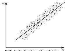
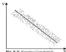
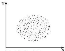
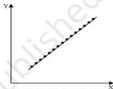
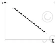
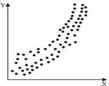
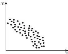
Figs 6.1, 6.2, 6.4 and 6.5 form the linear family; Fig. 6.3 shows no correlation; the last two are non-linear. The distinction decides the whole method.
Karl Pearson’s coefficient measures only linear relationships, so on the curved patterns of Figs 6.6 and 6.7 its value is misleading; the chapter’s rule is therefore to examine the scatter diagram before calculating any coefficient — the diagram tells you whether a numerical measure is appropriate at all (NCERT, p. 77).
Karl Pearson’s coefficient: the formula family and covariance
Karl Pearson’s coefficient of correlation — also called the product moment correlation coefficient or the simple correlation coefficient — gives a precise numerical value of the degree of linear relationship between two variables X and Y (NCERT, p. 77). It is built from three summary measures: the means, the variances, and a new one, the covariance of X and Y.
With N pairs of observations, the means and variances are (NCERT, p. 77):
\[ \bar{X} = \frac{\sum X}{N}, \qquad \bar{Y} = \frac{\sum Y}{N} \]
\[ \sigma_x^2 = \frac{\sum (X – \bar{X})^2}{N} = \frac{\sum X^2}{N} – \bar{X}^2, \qquad \sigma_y^2 = \frac{\sum (Y – \bar{Y})^2}{N} = \frac{\sum Y^2}{N} – \bar{Y}^2 \]
The standard deviations \( \sigma_x \) and \( \sigma_y \) are the positive square roots of these variances. The covariance of X and Y is defined as (NCERT, p. 79):
\[ \text{Cov}(X, Y) = \frac{\sum (X – \bar{X})(Y – \bar{Y})}{N} = \frac{\sum xy}{N} \]
where \( x = X – \bar{X} \) and \( y = Y – \bar{Y} \) are the deviations of the values from their own means. Note the sign logic: the sign of the covariance determines the sign of the correlation coefficient, the standard deviations are always positive, and a zero covariance means a zero correlation coefficient (NCERT, p. 79).
The coefficient itself appears in four equivalent forms. The deviation forms are (NCERT, p. 79):
\[ r = \frac{\sum xy}{N \sigma_x \sigma_y} \quad \dots (1) \]
\[ r = \frac{\sum (X – \bar{X})(Y – \bar{Y})}{\sqrt{\sum (X – \bar{X})^2} \sqrt{\sum (Y – \bar{Y})^2}} \quad \dots (2) \]
Forms (3) and (4) work directly with the raw sums \( \sum XY \), \( \sum X^2 \) and \( \sum Y^2 \); they are collected in the formula sheet below.
Whatever form you choose, the validity condition is identical: use Karl Pearson’s r only for linear relations. On non-linear data of the Fig. 6.6 / 6.7 type the coefficient is misleading (NCERT, p. 77). That fixes the working order: draw the scatter first, then calculate.
Properties of r: the rules that catch calculation errors
The properties of r are not abstract theory — several exist purely to catch arithmetic slips. The table compresses the chapter’s property list (NCERT, pp. 79–80):
| Property | What it means | How it helps you |
|---|---|---|
| r has no unit — it is a pure number | Units of measurement are not part of r; height in feet and weight in kg could give r = 0.7. The units cancel when covariance is divided by the product of the standard deviations | Never attach a unit to r in your answer |
| Negative r means an inverse relation | When one variable changes, the other changes in the opposite direction — commodity price rises while its demand falls | Check the sign of r against common sense |
| Positive r means the same direction | Both move together — when the price of coffee (a substitute for tea) rises, the demand for tea also rises | Check the sign of r against common sense |
| The range is \( -1 \leq r \leq 1 \) | The value of the correlation coefficient lies between minus one and plus one | An r outside this range signals an error in calculation |
| Change of origin and scale leaves r unchanged | For \( U = (X – A)/h \) and \( V = (Y – C)/k \) with h and k of the same sign, \( r_{uv} = r_{xy} \) | This property makes the step deviation method valid |
| r = 0 means uncorrelated | There is no linear relation between the variables — but other types of relation may exist | Never conclude “no relation” from r = 0; check for curves |
| r = 1 or r = -1 is perfect | There is an exact linear relation | Only possible when points lie exactly on a line |
| High means strong, low means weak | Values close to +1 or -1 indicate a strong linear relation; values close to zero a weak one | The sign shows direction; the absolute value shows strength |
The chapter pauses here to warn that statistical methods are no substitute for common sense (NCERT, p. 80).
Its illustration: in epidemic-hit villages, the correlation between the number of deaths and the number of doctors sent was positive — not because doctors raise death rates, but because many cases were already terminal, the benefit of medical care appears only after time, and a tsunami raised the death toll further. Understand the data before you calculate or interpret r.
Reading r: interpretation anchors
Read every value of r in two parts — the sign for direction, the absolute value for strength. The textbook’s examples (NCERT, p. 82):
| Value of r | Direction | Strength | What it looks like in practice |
|---|---|---|---|
| 0.1 | positive | weak | Scores in English and Statistics are positively related, but a high English score does not guarantee a high Statistics score |
| 0.9 | positive | strong | A high English score is almost always accompanied by a high Statistics score |
| -0.9 | negative | strong | A large vegetable supply in the mandi is accompanied by a much lower price |
| -0.1 | negative | weak | A large supply is accompanied by a lower price, but only slightly — the extent of the fall depends on the absolute value of r |
Keep r’s identity ready with the mnemonic BINS: Between -1 and 1 (the range), Inverse direction when negative (the sign), No unit (a pure number), Size — the absolute value — shows strength.
Step deviation method: taming large values
When the values of the variables are large, the burden of calculation can be reduced considerably by using the property that r is independent of change of origin and scale. The shortcut is the step deviation method (NCERT, p. 83). Choose assumed means A and C and common factors h and k, and transform the variables:
\[ U = \frac{X – A}{h}, \qquad V = \frac{Y – C}{k} \]
where A and C are assumed means of X and Y, and h and k are common factors with the same sign. Then \[ r_{UV} = r_{XY} \]
The correlation of the transformed variables equals the correlation of the original ones, because subtracting a constant shifts all values equally and dividing by a common factor rescales them uniformly — relative positions do not change.
The chapter’s Example 2 applies the method to the price index and money supply and obtains r = 0.98, a strong positive association that is an important premise of monetary policy: when the money supply grows, the price index also rises (NCERT, p. 83). The solved examples below run the same procedure on different data.
One practical caution: choose A, C, h and k so that U and V come out as small integers. If the transformed values are as awkward as the originals, the method has defeated its own purpose.
Spearman’s rank correlation: when only ranks exist
Spearman’s rank correlation, developed by the British psychologist C. E. Spearman, works on the ranks of the items rather than their measured values (NCERT, p. 83). The chapter gives four situations where it is the right tool (NCERT, pp. 83–84):
- Precise measurement is impossible. In a remote village with no measuring rods or weighing machines, students cannot be measured for height and weight — but they can certainly be ranked by each.
- One or both variables are attributes — qualities such as fairness, honesty or beauty that cannot be measured numerically, only ranked relatively.
- The direction of the relation is clear but non-linear — scatters of the Fig. 6.6 / 6.7 type.
- The data contain extreme values. Ranks are not affected by extremes, so Spearman’s coefficient is more robust here than Pearson’s.
The formula uses D, the deviation between the ranks assigned to an item on the two variables, and n, the number of observations (NCERT, p. 84):
\[ r_s = 1 – \frac{6 \sum D^2}{n^3 – n} \]
Interpretation matches r exactly: r_s also lies between -1 and 1, positive when the ranks move together and negative when they move in opposite directions. The chapter is honest about the cost, though: rank correlation is generally not as accurate as the ordinary method, because ranks discard the information in the size of the gaps between values (NCERT, p. 84).
Memory device: “Six D squares drag down the one.” Perfect agreement is 1; every rank gap D is squared, so large gaps hurt far more than small ones; the 6 is fixed; and dividing by \( n^3 – n \) scales the penalty to the number of observations.
Calculation falls into three situations (NCERT, p. 84):
Case 1: ranks are already given
Find D for each item, square it, add the squares, and substitute into the formula. The chapter’s beauty-contest example compares three judges and finds r_s = 0.3 between judges A and B, 0.5 between A and C, and -0.4 between B and C — so judges A and C share the closest perception of beauty (NCERT, p. 85).
Case 2: ranks must be worked out from raw data
Rank the values first, giving the highest value rank 1 — the convention used throughout the chapter — and rank both variables in the same direction. Then proceed exactly as in Case 1 (NCERT, p. 85).
Case 3: ranks repeat
When two or more items tie, each receives the average of the ranks they would have occupied, and the next item gets the rank that follows the ranks already assumed (NCERT, p. 86). Because the plain formula is then distorted, a correction term enters the bracket for every tied group:
\[ r_s = 1 – \frac{6 \left[ \sum D^2 + \frac{m_1^3 – m_1}{12} + \frac{m_2^3 – m_2}{12} + \cdots \right]}{n(n^2 – 1)} \]
where \( m_1, m_2, \dots \) are the sizes of the tied groups (NCERT, p. 86). In the chapter’s Case 3 illustration, Y = 50 appears three times at what would have been ranks 9, 10 and 11; all three get the average rank 10, the correction totals \( (3^3 – 3)/12 + (2^3 – 2)/12 = 2.5 \), and the result is r_s = 0.30 (NCERT, p. 86).
Choosing the right tool: scatter, Pearson or Spearman?
The chapter offers three techniques (NCERT, p. 76), and the recurring confusion is which one to apply. This table settles it:
| Tool | What it gives you | Limitation | Use it when |
|---|---|---|---|
| Scatter diagram | A visual form of any relationship — linear or not; shows direction and closeness | Gives no numerical value | Always — as the first step, before any coefficient |
| Karl Pearson’s r | A precise, unit-free number for the linear relationship | Misleading on curved (non-linear) patterns | The scatter hugs a line and the data are precisely measured |
| Spearman’s r_s | A number that works with ranks, attributes, one-directional curves and extreme values | Less accurate than r on precise data because ranks ignore gap sizes | Only ranks are possible, or the pattern is curved but one-directional |
Takeaway in one line: draw the scatter first. If the points hug a straight line, use Karl Pearson’s r; if you only have ranks, or the pattern is curved but one-directional, use Spearman’s r_s.
Formula sheet: every formula with symbol meanings
All the chapter’s formulas in one place for last-minute revision. Every line matches the chapter’s own presentation — verify any doubtful expression against the official textbook PDF for Chapter 6.
Building blocks: means, variances, covariance (NCERT, pp. 77–79) \[ \bar{X} = \frac{\sum X}{N}, \qquad \bar{Y} = \frac{\sum Y}{N} \]
\[ \sigma_x^2 = \frac{\sum (X – \bar{X})^2}{N} = \frac{\sum X^2}{N} – \bar{X}^2, \qquad \sigma_y^2 = \frac{\sum (Y – \bar{Y})^2}{N} = \frac{\sum Y^2}{N} – \bar{Y}^2 \]
\[ \text{Cov}(X, Y) = \frac{\sum xy}{N}, \quad \text{where } x = X – \bar{X} \text{ and } y = Y – \bar{Y} \]
Karl Pearson’s r — four equivalent forms (NCERT, p. 79) \[ r = \frac{\sum xy}{N \sigma_x \sigma_y} \quad \dots (1) \]
\[ r = \frac{\sum (X – \bar{X})(Y – \bar{Y})}{\sqrt{\sum (X – \bar{X})^2} \sqrt{\sum (Y – \bar{Y})^2}} \quad \dots (2) \]
\[ r = \frac{\sum XY – \frac{(\sum X)(\sum Y)}{N}}{\sqrt{\sum X^2 – \frac{(\sum X)^2}{N}} \sqrt{\sum Y^2 – \frac{(\sum Y)^2}{N}}} \quad \dots (3) \]
\[ r = \frac{N \sum XY – (\sum X)(\sum Y)}{\sqrt{N \sum X^2 – (\sum X)^2} \sqrt{N \sum Y^2 – (\sum Y)^2}} \quad \dots (4) \]
Step deviation transformation (NCERT, p. 83) \[ U = \frac{X – A}{h}, \qquad V = \frac{Y – C}{k}, \qquad r_{UV} = r_{XY} \]
Spearman’s rank correlation (NCERT, pp. 84, 86) \[ r_s = 1 – \frac{6 \sum D^2}{n^3 – n} \]
\[ r_s = 1 – \frac{6 \left[ \sum D^2 + \frac{m_1^3 – m_1}{12} + \frac{m_2^3 – m_2}{12} + \cdots \right]}{n(n^2 – 1)} \]
Symbol key
| Symbol | Meaning | Unit |
|---|---|---|
| X, Y | The two variables under study | Original units of the data |
| N | Number of pairs of observations (for rank correlation, n is used) | Count |
| \( x = X – \bar{X} \), \( y = Y – \bar{Y} \) | Deviations of the values from their means | Same units as X and Y |
| \( \sigma_x, \sigma_y \) | Standard deviations of X and Y, the positive square roots of the variances | Same units as X and Y |
| r | Karl Pearson’s coefficient of correlation | None — pure number |
| A, C | Assumed means of X and Y in the step deviation method | Same units as X and Y |
| h, k | Common factors of the same sign in the step deviation method | Same units as X and Y |
| \( r_s \) | Spearman’s rank correlation coefficient | None — pure number |
| n | Number of observations in the rank data | Count |
| D | Deviation between the ranks assigned to an item on the two variables | Rank units |
| m | Size of a tied group of ranks | Count |
Solved examples: all three methods, step by step
Three complete calculations on original data — work through each with a pen. Every example ends with direction and strength stated separately; that two-part conclusion is the complete interpretation of any coefficient.
Example 1: Karl Pearson’s coefficient by the deviation method
Step 1: Data: X = hours of study per week and Y = class-test score out of 20 for 6 students.
Use formula (2): \( r = \frac{\sum (X – \bar{X})(Y – \bar{Y})}{\sqrt{\sum (X – \bar{X})^2} \sqrt{\sum (Y – \bar{Y})^2}} \).
Step 2: Find the means: \( \bar{X} = 36/6 = 6 \) hours and \( \bar{Y} = 60/6 = 10 \) (score units, since scores are out of 20).
Step 3: Build the working table with deviations \( x = X – 6 \) and \( y = Y – 10 \):
| X | Y | \( x = X – \bar{X} \) | \( y = Y – \bar{Y} \) | \( x^2 \) | \( y^2 \) | \( xy \) |
|---|---|---|---|---|---|---|
| 1 | 8 | \( -5 \) | \( -2 \) | 25 | 4 | 10 |
| 3 | 10 | \( -3 \) | 0 | 9 | 0 | 0 |
| 5 | 5 | \( -1 \) | \( -5 \) | 1 | 25 | 5 |
| 7 | 12 | 1 | 2 | 1 | 4 | 2 |
| 9 | 9 | 3 | \( -1 \) | 9 | 1 | \( -3 \) |
| 11 | 16 | 5 | 6 | 25 | 36 | 30 |
Step 4: From the table: \( \sum x^2 = 70 \), \( \sum y^2 = 70 \), \( \sum xy = 44 \).
Substitute into formula (2):
\[ r = \frac{44}{\sqrt{70 \times 70}} = \frac{44}{70} \approx 0.63 \]
Final answer: \( r \approx 0.63 \) — a moderate positive correlation: more study hours go with higher class-test scores.
Example 2: Step deviation method (price vs quantity demanded)
Step 1: Data: X = price of a vegetable in ₹ per kg and Y = quantity demanded per day in kg.
Choose \( A = 10 \), \( h = 10 \), \( C = 90 \), \( k = 5 \), giving \( U = (X – 10)/10 \) and \( V = (Y – 90)/5 \).
Step 2: Transform the data and build the table.
The transformed values come out as small integers, which is the whole point of the method:
| X | Y | U | V | \( U^2 \) | \( V^2 \) | \( UV \) |
|---|---|---|---|---|---|---|
| 10 | 90 | 0 | 0 | 0 | 0 | 0 |
| 20 | 55 | 1 | \( -7 \) | 1 | 49 | \( -7 \) |
| 30 | 60 | 2 | \( -6 \) | 4 | 36 | \( -12 \) |
| 40 | 75 | 3 | \( -3 \) | 9 | 9 | \( -9 \) |
| 50 | 35 | 4 | \( -11 \) | 16 | 121 | \( -44 \) |
Step 3: Column sums: \( \sum U = 10 \), \( \sum V = -27 \), \( \sum U^2 = 30 \), \( \sum V^2 = 215 \), \( \sum UV = -72 \).
Step 4: Substitute these into formula (3) applied to U and V:
\[ r = \frac{\sum UV – \frac{(\sum U)(\sum V)}{N}}{\sqrt{\sum U^2 – \frac{(\sum U)^2}{N}} \sqrt{\sum V^2 – \frac{(\sum V)^2}{N}}} \]
\[ = \frac{-72 – \frac{(10)(-27)}{5}}{\sqrt{30 – \frac{10^2}{5}} \sqrt{215 – \frac{(-27)^2}{5}}} = \frac{-72 + 54}{\sqrt{30 – 20} \sqrt{215 – 145.8}} = \frac{-18}{\sqrt{10} \sqrt{69.2}} \approx -0.68 \]
Final answer: \( r \approx -0.68 \) — a moderate negative correlation: as the price rises, the quantity demanded tends to fall. The demand rise at ₹40 (a festival-buying week) breaks the straight-line pattern and weakens the coefficient.
Example 3: Spearman’s rank correlation with a repeated rank
Step 1: Data: Mathematics scores (X) and Statistics scores (Y) of 8 students.
Rank both variables in the same direction, highest score = rank 1.
Step 2: Handle the tie.
The value 65 appears twice in Y; the two tied items would have occupied ranks 2 and 3, so each receives the average rank 2.5.
The correction for this one tied group is \( (2^3 – 2)/12 = 0.5 \).
Step 3: Work out D (rank of X minus rank of Y) and \( D^2 \):
| X | Y | Rank of X | Rank of Y | D | \( D^2 \) |
|---|---|---|---|---|---|
| 45 | 30 | 8 | 8 | 0 | 0 |
| 52 | 42 | 7 | 7 | 0 | 0 |
| 60 | 50 | 6 | 5 | 1 | 1 |
| 68 | 46 | 5 | 6 | \( -1 \) | 1 |
| 74 | 65 | 4 | 2.5 | 1.5 | 2.25 |
| 81 | 58 | 3 | 4 | \( -1 \) | 1 |
| 88 | 65 | 2 | 2.5 | \( -0.5 \) | 0.25 |
| 95 | 72 | 1 | 1 | 0 | 0 |
Step 4: Column sum: \( \sum D^2 = 5.5 \).
Apply the repeated-rank formula, adding the correction inside the bracket:
\[ r_s = 1 – \frac{6(5.5 + 0.5)}{8^3 – 8} = 1 – \frac{36}{504} \approx 0.93 \]
Final answer: \( r_s \approx 0.93 \) — a strong positive rank correlation: students who score high in Mathematics tend to score high in Statistics.
Notice the common shape of all three answers: direction first (positive or negative), then strength (moderate, strong), with r itself kept unit-free.
Common mistakes: what students write vs what is correct
Every row below is a pattern that appears in real student solutions. Correct each one the moment you see it.
| Mistake | Correct rule | How to check your answer |
|---|---|---|
| “r = 0, so the two variables are independent” | r = 0 means only that there is no LINEAR relation. A U-shaped pattern gives r = 0 while Y clearly changes with X — the chapter’s exercise-19 data (X = -3 to 3, Y = 9, 4, 1, 1, 4, 9) is exactly this case | Plot the scatter; if a curve is visible, r = 0 is the expected, correct result |
| “High correlation proves one variable causes the other” | Correlation is covariation, not causation. Ice-cream sales and drowning deaths both rise with temperature without causing each other | Ask: could a third variable be driving both? In summer data it usually can |
| “r = 1.6 means a very strong relation” | Impossible — r lies between \( -1 \) and 1. Any value outside the range signals an error in calculation | Re-add the sums: \( \sum x^2 \), \( \sum y^2 \), \( \sum xy \) (or \( \sum U^2 \), \( \sum V^2 \), \( \sum UV \) in the step deviation method) |
| “I skipped the correction for repeated ranks” | Tied items take the average of the ranks they would have occupied, and the bracket needs \( \sum (m^3 – m)/12 \), otherwise \( r_s \) is wrong | Count each tied group of size m and add its \( (m^3 – m)/12 \) to \( \sum D^2 \) before multiplying by 6 |
| “I applied Pearson’s r to a curved scatter” | Pearson’s r measures only linear relationships; on a curve it is misleading | Look at the scatter first; for a one-directional curve switch to rank correlation |
| “-0.9 is weaker than 0.1” | Strength is the absolute value; the sign shows only direction | Compare absolute values, not signed values |
| “I ranked one variable from highest and the other from lowest” | Rank both variables in the same direction (highest = 1), otherwise the sign of \( r_s \) flips | Verify both rank columns assign rank 1 to the highest value of each variable |
Answering the chapter’s exercises: writing complete answers
The exercise list runs from Q1 to Q20 (NCERT, pp. 88–89). The patterns below show what a complete answer contains; the full exercise text is available from the official NCERT textbook portal.
Short concept checks (Q1–Q6). Each of the first six questions maps to exactly one property in the tables above: the unit of r, the range of r, the meaning of a positive r, the meaning of r = 0, the one tool that can reveal any type of relationship, and the relative accuracy of simple versus rank correlation on precise data.
Answer each in one sentence that names the property explicitly — a paraphrase that changes its meaning loses the point.
Reasoning questions (Q7–Q12, Q16, Q17). Open with the principle, support it with one short example from the chapter, and close with a one-line conclusion.
- Q7: lead with why r beats covariance — covariance carries the product of the units of X and Y, so its size depends on the units; r divides covariance by \( \sigma_x \sigma_y \), removing units and fixing the range to \( -1 \) to 1.
- Q8 and Q16: state the range and the three anchor values — r outside \( -1 \) to 1 is impossible for any data; r = 1, \( -1 \) and 0 mean perfect positive, perfect negative and no linear relation.
- Q9: correlation is covariation, not causation — no coefficient implies cause and effect.
- Q10 and Q12: rank correlation becomes the more precise tool when measurement is imprecise, when attributes are involved, or when the relation is one-directional but non-linear; the simple coefficient cannot measure every type of relationship because it is limited to linear ones.
- Q11: r = 0 means no linear relation, not independence — a U-shaped relation changes Y while giving r = 0, as exercise-19 data show.
- Q17: rank correlation works on ranks, not values, and discards the size of the gaps — that is why it generally differs from Pearson’s coefficient.
Calculation questions (Q18–Q20). The complete-answer format is: formula → working table → substitution → value → interpretation. Use columns X, Y, \( x^2 \), \( y^2 \), \( xy \) for Pearson’s method and ranks, D, \( D^2 \) for Spearman’s. The chapter prints the answers — r = 0.603 for Q18, r = 0 for Q19 and r = 1 for Q20 — so use them to check the arithmetic.
Q19 is the case where r = 0 is correct and meaningful: the symmetric U-shaped values make the positive and negative products cancel in the covariance sum.
Collect-and-interpret questions (Q13, Q14) and the list question (Q15).
For Q13 and Q14, state the data you would collect (five vegetable prices over a week; each classmate’s measured height paired with the height they give when asked), name the tool, and give a template interpretation: a positive coefficient means the two variables move together across the observations, a negative one means they move in opposite directions.
For Q15, list variables where accurate measurement is difficult — the chapter’s own examples are intelligence, honesty, beauty and physical appearance — and link that list to Spearman’s method.
Revision recap: the whole chapter on one page
The chapter closes with six recap points, and they are the ready-to-use summary of everything above (NCERT, p. 87):
- Correlation analysis studies the relation between two variables.
- Scatter diagrams give a visual presentation of the nature of the relationship.
- Karl Pearson’s coefficient r measures numerically only linear relationships; r lies between \( -1 \) and 1.
- When variables cannot be measured precisely, Spearman’s rank correlation can measure the relationship numerically.
- Repeated ranks need correction factors.
- Correlation does not mean causation — it only means covariation.
And the concept map — each idea, its key fact, and the moment it matters:
| Concept | Key formula or fact | When it matters |
|---|---|---|
| Covariance | \( \sum xy / N \); its sign fixes the sign of r | Understanding why r will be positive or negative before you calculate |
| Karl Pearson’s r | \( r = \sum xy / (N \sigma_x \sigma_y) \), unit-free, between \( -1 \) and 1 | Precisely measured, linear data |
| Step deviation | \( U = (X – A)/h \), \( V = (Y – C)/k \); \( r_{UV} = r_{XY} \) | Large or awkward values — lightening the arithmetic |
| Spearman’s r_s | \( r_s = 1 – 6 \sum D^2 / (n^3 – n) \) | Ranks, attributes, one-directional curves, extreme values |
| Tie correction | Add \( \sum (m^3 – m)/12 \) inside the bracket | Whenever ranks repeat |
For the chapters around this one, browse the full Class 11 notes hub or the complete CBSE notes library.
Frequently asked questions on correlation (with answers)
Does zero correlation mean the two variables are independent?
No. r = 0 means only that there is no linear relationship between them. A non-linear relation can still exist: the chapter’s exercise-19 data — X = -3, -2, -1, 1, 2, 3 against Y = 9, 4, 1, 1, 4, 9 — form a U-shape in which Y clearly changes with X, yet r = 0 because the positive and negative products cancel in the covariance sum.
Why is r preferred to covariance as a measure of association?
Because covariance carries the product of the units of X and Y, its size depends on the units chosen, so it cannot be compared across datasets. Dividing the covariance by \( \sigma_x \sigma_y \) removes the units and fixes the value to the range \( -1 \) to 1 — that standardised, unit-free number is r.
When should I use Spearman’s rank correlation instead of Karl Pearson’s coefficient?
Use it when precise measurement is impossible so only ranks can be assigned, when one variable is an attribute such as honesty or beauty, when the relation is clearly one-directional but non-linear, or when the data contain extreme values — ranks are not affected by extremes (NCERT, pp. 83–84).
What is the correction factor in Spearman’s rank correlation and when is it needed?
It is the term \( (m^3 – m)/12 \) added inside the formula’s bracket, one term for each tied group of size m. It is needed whenever ranks repeat: tied items receive the average of the ranks they would have occupied, and the plain formula would be distorted without this adjustment (NCERT, p. 86).
Can Karl Pearson’s coefficient r measure non-linear relationships?
No. r measures only the degree of linear relationship. On a curved scatter of the Fig. 6.6 / 6.7 type its value is misleading — which is why the chapter insists on examining the scatter diagram before calculating r (NCERT, p. 77).
Is rank correlation more accurate than simple correlation for precisely measured data?
No — the opposite. Rank correlation is generally not as accurate as the ordinary method, because ranks discard the information contained in the size of the gaps between values. Precisely measured data call for Karl Pearson’s coefficient (NCERT, p. 84).
Reference: NCERT Class 11 Statistics for Economics textbook, chapter Correlation.
Explore Class 11 Economics Notes
- Class 11 Economics Notes
- Class 11 CBSE Notes
- CBSE Notes for Classes 1 to 12
- Previous: Measures of Central Tendency
Class 11 Economics on LearnCBSE:
Related chapters:
- Why Economics? notes
- Organisation of Data notes
Official source: download the NCERT textbook free from ncert.nic.in.