
This is NCERT Class 12 Computer Science Chapter 9, Structured Query Language (SQL) — the chapter that shows you how to actually build a relational database and talk to it. The chapter runs to roughly 50 printed pages of the textbook, and every command in it runs on MySQL, the free RDBMS the book uses throughout.
It builds directly on the schema and key concepts introduced in Chapter 8, Database Concepts — so if you know what a relation and a primary key are, you are ready for this chapter. The official chapter PDF is one click below, and the rest of the page explains what you will find inside it.
- Download the SQL Class 12 PDF
- Chapter 9 at a glance
- What this chapter covers
- Key ideas in the chapter, explained
- Figures in the chapter, explained
- Definitions you will need
- Common mistakes — and Think and Reflect answers
- How to practise SQL from this chapter
- Chapter recap in one read
- Related chapters and resources
- Sources and data verification
- Frequently asked questions
Download the Structured Query Language (SQL) Class 12 PDF
NCERT publishes the textbook free of charge, and you can download the official NCERT Structured Query Language (SQL) Class 12 Computer Science Chapter 9 PDF from the NCERT textbook portal and keep it beside this page while you practise the queries.
This is the standard NCERT Computer Science book for Class 12 — the edition that also contains Database Concepts as Chapter 8 and Computer Networks as Chapter 10.
Reference: NCERT Class 12 Computer Science textbook, chapter 9, official edition on ncert.nic.in.
Not ready to download anything yet? The rest of this page walks through every section of the chapter — what each command family does, which figure shows what, and how the exercises work.
| What the chapter holds | Count | Where it is used |
|---|---|---|
| Printed pages | 50 | |
| Sections in the chapter | 32 | |
| Figures with NCERT captions | 6 | |
| Tables | 78 | |
| Worked examples | 4 | solved step by step in our NCERT Solutions |
| Exercise questions | 3 | answered in our NCERT Solutions |
| Activities | 15 | |
| Official NCERT PDF | Download the chapter PDF | the chapter exactly as NCERT publishes it |
Chapter 9 at a glance
The table below is pulled straight from the textbook and counts what Chapter 9 actually contains — numbered sections, figures, activities, worked examples and exercise questions. Skim it before you start, so you know how much of the chapter is concept-building and how much is typing queries into MySQL.
What this chapter covers
Chapter 9 is organised into eleven numbered parts, and each one adds a piece of the SQL skill set:
- 9.1 Introduction (p. 131) — where the chapter sits after the RDBMS concepts of Chapter 8.
- 9.2 What SQL is, and installing MySQL (p. 131–132) — SQL as the query language of relational systems, the
mysql>prompt, and the three house rules for writing statements. - 9.3 Data types and constraints (p. 133–134) — CHAR, VARCHAR, INT, FLOAT, DATE, and the constraints NOT NULL, UNIQUE, DEFAULT, PRIMARY KEY, FOREIGN KEY.
- 9.4 SQL for Data Definition (p. 134–141) — CREATE DATABASE, CREATE TABLE, DESCRIBE, ALTER TABLE in its many forms, and DROP.
- 9.5 SQL for Data Manipulation (p. 141–144) — INSERT INTO with and without column names, plus the foreign-key caution.
- 9.6 SQL for Data Query (p. 144–153) — the SELECT statement with its clauses: alias, DISTINCT, WHERE, BETWEEN, IN, ORDER BY, IS NULL and LIKE.
- 9.7 Data Updation and Deletion (p. 154–155) — UPDATE and DELETE, with the warning about a missing WHERE clause.
- 9.8 Functions in SQL (p. 156–166) — single-row functions (Math, String, Date and Time) and aggregate functions (MAX, MIN, AVG, SUM, COUNT).
- 9.9 GROUP BY clause (p. 167–168) — grouping rows by common values and filtering groups with HAVING.
- 9.10 Operations on Relations (p. 169–171) — UNION, INTERSECT, MINUS and Cartesian product, with the degree-and-cardinality rule.
- 9.11 Using Two Relations in a Query (p. 172–175) — comma-separated FROM, JOIN … ON and NATURAL JOIN, with table aliases.
The chapter practises on three running databases: StudentAttendance (the school database from Chapter 8) is built in sections 9.4–9.5; OFFICE, an organisation database with an EMPLOYEE table, is used for SELECT practice in section 9.6; and CARSHOWROOM, with four relations, powers the functions and GROUP BY sections from 9.8 onward. The chapter ends with a SUMMARY (p. 175) and an EXERCISE of eight questions (p. 176–180).
Key ideas in the chapter, explained
After Chapter 8 explained what a relational database is — tables, rows, primary and foreign keys — this chapter shows you how to build one and ask questions of it. The whole chapter is practical: you type SQL statements into MySQL, and MySQL answers back with tables.
What SQL is and the two sides of the language
SQL (Structured Query Language) is the query language used by the major relational database systems — the book names MySQL, Oracle, SQL Server and PostgreSQL (p. 131). The property that makes SQL powerful is that it is declarative: you say what data you want (“all employees in department D01”), not how to fetch it. The DBMS works out the fetching.
Three habits to keep from the very start (p. 132): every statement ends with a semicolon (;); SQL is case insensitive, so salary and SALARY are the same column name; and a multiline statement continues at the -> prompt, with the semicolon only after the last line.
The chapter is organised around a two-way split that you should keep in mind through every section:
- DDL (Data Definition Language) — statements that define or change the structure of a database:
CREATE,ALTER,DROP(p. 134). - DML (Data Manipulation Language) — statements that work on the data itself:
INSERT,SELECT,UPDATE,DELETE(p. 141).
Data types and constraints in MySQL
Before you create a single table you must decide, for every column, what kind of value it will hold (its data type) and what rules protect it (its constraints). These two design choices are the subject of section 9.3.
| Data type | What it stores | The key behaviour (p. 133) |
|---|---|---|
| CHAR(n) | Fixed-length text | Declaring CHAR(10) reserves 10 spaces; a shorter value is padded with spaces on the right. |
| VARCHAR(n) | Variable-length text | VARCHAR(30) allows up to 30 characters but stores only what you type. |
| INT | Whole numbers, 4 bytes | Unsigned range 0 to 4,294,967,295; bigger values need BIGINT. |
| FLOAT | Numbers with decimal points | Each value occupies 4 bytes. |
| DATE | Dates in ‘YYYY-MM-DD’ format | Supported range ‘1000-01-01’ to ‘9999-12-31’. |
Constraints (p. 134) are restrictions on the values a column may take: NOT NULL forbids missing values, UNIQUE forbids duplicates, DEFAULT supplies a value when none is given, PRIMARY KEY uniquely identifies each row, and FOREIGN KEY refers to a primary key in another table.
The book’s own Think and Reflect asks which two constraints together behave like a primary key — the answer is NOT NULL + UNIQUE (p. 134).
The CHAR-versus-VARCHAR judgement matters for real tables. For fixed-length codes such as a 12-digit Aadhaar number or a 10-digit mobile number, CHAR is the better choice: no arithmetic is ever done on these values, and CHAR avoids variable-length storage overhead (p. 137).
Creating and changing tables: the DDL statements
DDL is how an empty database becomes a working schema. The chapter builds the StudentAttendance database step by step, and you should learn the commands in that same order.
CREATE DATABASE StudentAttendance;thenUSE StudentAttendance;thenSHOW TABLES;to confirm the database is empty (p. 134).CREATE TABLEwith one line per attribute — name, data type, constraint — separated by commas and ending with a semicolon (p. 135).DESCRIBE tablename;to view a table’s structure — its fields, types, NULL rules and keys (p. 137).ALTER TABLEfor schema changes: add a primary key, add a foreign key, add UNIQUE, add a new attribute, modify a data type, modify to NOT NULL, add a DEFAULT value, drop an attribute, or drop the primary key (p. 138–140).DROP TABLE tablename;orDROP DATABASE databasename;to remove structure permanently — the book warns this cannot be undone (p. 141).
Three conditions must hold when you add a foreign key (p. 138): the referenced table must already exist, the referenced attribute must be part of its primary key, and the data types of the referenced and referencing attributes must match. In the chapter’s example, STUDENT (the referencing table) points to GUARDIAN (the referenced table) through the common attribute GUID.
Filling and changing data: the DML statements
Creating a table only builds its structure — the table has no data yet. DML puts data in, changes it and removes it, and this is where the chapter’s first serious caution appears.
INSERT INTO tablename VALUES (...);— one value per column, in the table’s column order. Use the column-name formINSERT INTO tablename (col1, col2) VALUES (...);when some columns should stay NULL or take a default value (p. 141–142).- Text and date values go inside single quotes; numbers do not —
'Amit Ahuja','2003-05-15', but5711492685(p. 142). UPDATE tablename SET column = value WHERE condition;— modifies existing rows (p. 154).DELETE FROM tablename WHERE condition;— removes rows (p. 155).
The danger the book repeats twice: miss the WHERE clause in an UPDATE or DELETE, and every row is changed or deleted. There is also a foreign-key order to respect: populate the referenced table (GUARDIAN) before the referencing table (STUDENT) (p. 141).
Querying with SELECT
SELECT is the chapter’s largest section because asking questions of data is the whole point of a database. Learn one shape first — SELECT columns FROM table WHERE condition; (p. 144) — and then add each clause to it. Every clause below is practised on the OFFICE database’s EMPLOYEE table (p. 145).
- Alias AS — renames a column in the output only; the table itself is unchanged. An alias containing a space must be quoted:
'Annual Income'(p. 146). - DISTINCT — removes repeated values, e.g. listing each department once (p. 147).
- WHERE — conditions with relational operators
<,<=,>,>=,=,!=combined with AND, OR and NOT; string values in quotes (p. 148). - BETWEEN — an inclusive range:
Salary BETWEEN 20000 AND 50000includes both boundary values (p. 148–149). - IN / NOT IN — matches any value in a list:
DeptId IN ('D01', 'D02', 'D04')(p. 150). - ORDER BY — sorts the output, ascending by default, with DESC for descending (p. 151).
- IS NULL / IS NOT NULL — NULL means a missing or unknown value, not zero;
5 + NULLgives NULL, and you never test with= NULL(p. 151–152). - LIKE — pattern matching with two wildcards:
%for zero or more characters and_for exactly one (p. 152–153).
Functions: single-row and aggregate
Functions let you transform values inside a query instead of fetching them raw. The chapter switches to the richer CARSHOWROOM database here — four relations named INVENTORY, CUSTOMER, SALE and EMPLOYEE (p. 156) — so that the examples have realistic data.
There are two families with a simple difference. Single-row functions take one value and return one value per row: Math (POWER, ROUND, MOD), String (UCASE/LCASE, MID/SUBSTRING/SUBSTR, LENGTH, LEFT, RIGHT, INSTR, LTRIM/RTRIM/TRIM), and Date and Time (NOW, DATE, MONTH, MONTHNAME, YEAR, DAY, DAYNAME) (p. 158–164).
Aggregate functions take a whole column of records and return a single value: MAX, MIN, AVG, SUM, and both COUNT(*) and COUNT(column) (p. 165–166).
Two distinctions decide where each family is allowed. A single-row function can appear in SELECT, WHERE and ORDER BY; an aggregate function appears in the SELECT clause alone (p. 165). And COUNT(column) ignores NULL values while COUNT(*) counts every record — in the book’s MANAGER example, four records but only three names, so COUNT(MEMNAME) returns 3 (p. 166).
GROUP BY and HAVING
GROUP BY answers “per group” questions — how many cars each customer bought, how many employees each designation has. It collects rows that share the same value in a column so an aggregate can run on each group separately. HAVING then filters the groups, the way WHERE filters rows before grouping (p. 167–168).
Because HAVING completes the SELECT clause order, learn the sequence in one piece:
Find What Groups Have Ordered — FROM picks the table, WHERE filters rows, GROUP BY forms the groups, HAVING filters the groups, ORDER BY sorts the final result.
Set operations and joins on two tables
Real questions cut across tables — which students are in both Dance and Music? Two tools do this: set operations on whole relations, and joins that combine rows on matching attributes.
Set operations need a condition: both relations must have the same number of attributes and matching domains. UNION gives rows in either table (duplicates shown once), INTERSECT gives rows in both, MINUS gives rows in the first but not the second, and the Cartesian product gives every possible pair of rows (p. 169–171).
Two measures describe the result: degree is the number of columns and cardinality the number of rows. The book’s DANCE × MUSIC example — degree 3 and cardinality 4 crossed with degree 3 and cardinality 5 — yields degree 6 and cardinality 20: degrees add, cardinalities multiply (p. 171).
Queries on two tables come in three styles, and the chapter demonstrates all three on the UNIFORM and COST tables (p. 172–175):
| Method | Syntax | What changes in the result |
|---|---|---|
| Comma-separated FROM + WHERE | SELECT * FROM UNIFORM U, COST C WHERE U.UCode = C.UCode; |
Cartesian product filtered by the condition; the common column UCode appears twice. |
| JOIN … ON | SELECT * FROM UNIFORM U JOIN COST C ON U.UCode = C.UCode; |
Only matching pairs, joined inside the FROM clause; UCode still appears twice. |
| NATURAL JOIN | SELECT * FROM UNIFORM NATURAL JOIN COST; |
Same rows as the other two, but the duplicated common column is removed. |
Use table aliases (D for DANCE, M for MUSIC) to keep the query readable, remember that an aliased table can only be called by its alias inside that query, and note the rule that N tables need N − 1 joins on equality conditions.
In practice a join usually links a primary key in one table to a foreign key in another (p. 172–175).
Figures in the chapter, explained
The chapter carries six diagrams, and each one does a specific job. Reading them as you meet them makes the text around them click into place.
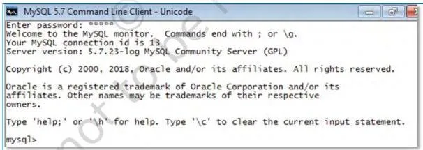
Figure 9.1 (p. 132) is a screenshot of the MySQL shell. The mysql> prompt is MySQL saying it is ready to accept SQL statements — everything in this chapter starts from this line. When you press Enter to continue a long statement, the prompt changes to -> until you end the statement with a semicolon.
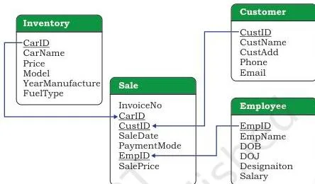
Figure 9.2 (p. 156) is a schema diagram — a map of the CARSHOWROOM database. Each box is a relation and each connecting line is a foreign-key link. SALE sits at the centre: it records which car (INVENTORY), which buyer (CUSTOMER) and which salesperson (EMPLOYEE).
This is where the schema idea from Chapter 8 becomes a working database, and it tells you in advance which attributes you will write in JOIN conditions later.
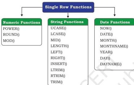
Figure 9.3 (p. 158) organises single-row functions into their three categories. The logic to remember is input–output: Math functions accept a numeric value and return a numeric value; String functions accept a character value and return a character or numeric value; Date and Time functions accept a date and return a number, a string or a date.
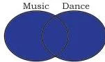
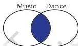
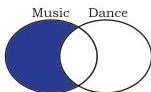
Figures 9.4, 9.5 and 9.6 (p. 169–171) are the same pair of overlapping circles drawn three ways, and they map exactly onto the chapter’s DANCE and MUSIC tables. Union shades all of both circles — the result table holds 7 rows, because students in both events appear only once. Intersection shades only the overlap — the result holds 2 rows, the students in both.
Difference shades one circle without the overlap — the result holds 3 rows, the students in one event only.
Definitions you will need
These are the terms the chapter uses constantly, in plainer words than the book, with the page where each is introduced.
| Term | Meaning |
|---|---|
| SQL (p. 131) | Structured Query Language — the query language used by MySQL and other relational database systems. |
| RDBMS (p. 131) | Relational Database Management System — software that stores and manages data as relations, or tables. |
| Query (p. 131) | A SQL statement, usually a SELECT, that retrieves data from a database. |
| DDL (p. 134) | Data Definition Language — statements that define or change structure: CREATE, ALTER, DROP. |
| DML (p. 141) | Data Manipulation Language — statements that work on data: INSERT, SELECT, UPDATE, DELETE. |
| Data type (p. 133) | The kind of value an attribute can hold, which also decides the operations allowed on it. |
| Constraint (p. 134) | A restriction on the values an attribute may take, used to keep data correct. |
| NULL (p. 151) | A special value meaning missing, unknown or not applicable — not the same as 0. |
| Primary key (p. 134) | The column (or columns) that uniquely identifies each row of a table. |
| Foreign key (p. 134) | A column in one table that refers to a primary key in another table. |
| Composite primary key (p. 136) | A primary key made of two or more columns together, like (AttendanceDate, RollNumber). |
| Degree (p. 135) | The number of columns (attributes) in a relation. |
| Cardinality (p. 171) | The number of rows (tuples) in a relation. |
| Alias (p. 146) | A temporary name for a column or table, valid only for the current query. |
| Wildcard characters (p. 152) | % (zero or more characters) and _ (exactly one character), used with LIKE. |
| Aggregate function (p. 165) | A function that works on a whole column of rows and returns one value — MAX, MIN, AVG, SUM, COUNT. |
Common mistakes — and the answers to Think and Reflect
The chapter flags its own traps inside cautions and Think and Reflect prompts. These are the errors that cost marks in practical work, so fix them before they happen.
| Mistake | Correct rule | How to check your answer |
|---|---|---|
| UPDATE or DELETE without a WHERE clause | WHERE limits the statement to matching rows; without it, every row is changed or deleted (p. 154–155). | Run the same SELECT with the WHERE clause first and count the rows; check the “Rows matched” line after UPDATE. |
Testing NULL with = NULL |
NULL is a missing value, not 0; test with IS NULL and IS NOT NULL. Any arithmetic with NULL gives NULL — 5 + NULL = NULL (p. 151). |
Use WHERE Bonus IS NULL; a = NULL condition returns no rows at all. |
| Inserting into a table with a foreign key before its referenced table | Fill the referenced table (GUARDIAN) first, then the referencing table (STUDENT) (p. 141). | Insert into STUDENT only after the GUID already exists in GUARDIAN; MySQL rejects the row otherwise. |
| Confusing CHAR and VARCHAR | CHAR pads with spaces to its declared length; VARCHAR stores only what is typed. Use CHAR for fixed-length codes like Aadhaar or phone numbers (p. 133, 137). | Compare LENGTH() on the same value stored in a CHAR(10) and a VARCHAR(10) column. |
| Leaving single quotes off text and date values | Text and dates sit inside ‘ ‘; numbers do not — 'Amit Ahuja', '2003-05-15', but 5711492685 (p. 142). |
Check every INSERT and WHERE: quoted values are strings or dates, unquoted values are numbers. |
| Expecting string comparison to be case sensitive | SQL is case insensitive — ‘Aaliya’ and ‘AALIYA’ match (p. 149). | WHERE Ename = 'aaliya' still finds the employee Aaliya. |
Three Think and Reflect prompts the book leaves open, answered:
- Which two constraints combine into a primary key? NOT NULL and UNIQUE applied together behave like a PRIMARY KEY — unique values that cannot be missing (p. 134).
- CHAR or VARCHAR for a contact number? CHAR, because a mobile number is fixed length (10 digits) and no arithmetic is ever performed on it, so CHAR’s padding costs nothing and avoids variable-length overhead (p. 137).
- What range fits in an INT column? The unsigned range the book states is 0 to 4,294,967,295 (p. 133). MySQL’s default signed INT runs from about −2.1 billion to +2.1 billion — the signed figure is the MySQL default rather than a figure NCERT states.
How to practise SQL from this chapter
The exercise on pages 176–180 contains eight questions, and they train three distinct skills. Knowing which skill each question practises tells you how to prepare for it.
| Exercise | Table(s) used | Skill it trains |
|---|---|---|
| 1 (p. 176) | None | Concepts and differences: RDBMS, ORDER BY vs GROUP BY, single-row vs aggregate functions, Cartesian product, ALTER vs UPDATE, DELETE vs DROP, naming the right function for a job. |
| 2 (p. 177) | None | Output prediction: POW, ROUND, LENGTH, YEAR/MONTH/DAY/MONTHNAME, LEFT/RIGHT/MID/SUBSTR. |
| 3 (p. 177) | MOVIE | Query writing: calculated columns with aliases, listing categories, cost ranges. |
| 4 (p. 178) | Sports TEAM, MATCH_DETAILS | Query writing: CREATE TABLE with data types and a primary key, then INSERT. |
| 5 (p. 178) | TEAM + MATCH_DETAILS | Query writing: two-table conditions, plus renaming a table and its attributes. |
| 6 (p. 179) | SCHOOLUNIFORM | Constraint correction: foreign-key checks and a rule that prices stay above zero. |
| 7 (p. 179) | Product | Query writing: GROUP BY, aggregates, UPDATE, DISTINCT. |
| 8 (p. 180) | CARSHOWROOM | Query writing: ALTER to add a column, UPDATE to fill it, aggregates with conditions. |
For output-prediction questions (Q2, and parts of Q7), a full answer writes the exact output table with its column headers. For query-writing questions, write the complete statement ending with a semicolon and use aliases exactly as the question demands.
A complete worked session on a new table
The five queries below are not from the book — they run on a fresh table, built with the same commands the chapter teaches. Create it, and the whole chapter falls into place.
CREATE TABLE LIBRARY (BCode CHAR(4), Title VARCHAR(50), Author VARCHAR(30), Price INT, IssueDate DATE);
| BCode | Title | Author | Price | IssueDate |
|---|---|---|---|---|
| B101 | The Guide | R.K. Narayan | 450 | 2023-06-12 |
| B102 | Wings of Fire | A.P.J. Abdul Kalam | 380 | 2023-07-03 |
| B103 | Discovery of India | R.K. Narayan | 520 | 2023-08-19 |
| B104 | Godan | Premchand | 340 | 2023-06-25 |
| B105 | My Experiments with Truth | M.K. Gandhi | 410 | 2023-09-01 |
| B106 | The White Tiger | Aravind Adiga | 550 | 2023-07-15 |
Query 1 — a range filter with AND. SELECT Title, Price FROM LIBRARY WHERE Price >= 400 AND Price <= 520; returns The Guide (450), Discovery of India (520) and My Experiments with Truth (410) — three rows, because both conditions must hold. BETWEEN 400 AND 520 would give the same result, since BETWEEN is inclusive at both ends.
Query 2 — an aliased calculated column. SELECT Title, Price, Price * 1.05 AS PriceWithTax FROM LIBRARY; adds a third column showing each price with 5% tax — 472.50, 399.00, 546.00, 357.00, 430.50, 577.50. The alias exists only in the output; the LIBRARY table itself is untouched.
Query 3 — ORDER BY. SELECT Title, Author FROM LIBRARY ORDER BY Price DESC; sorts the books from most to least expensive. Without DESC the same query sorts ascending, which is the default.
Query 4 — GROUP BY with HAVING. SELECT Author, COUNT(*) AS Books FROM LIBRARY GROUP BY Author HAVING COUNT(*) > 1; groups the six books by author and keeps only the groups with more than one book: R.K. Narayan, with 2. Every other author’s group is filtered out by HAVING.
Query 5 — a LIKE pattern. SELECT Title FROM LIBRARY WHERE Title LIKE '%the%'; matches The Guide and The White Tiger. The % wildcard stands for any characters before and after ‘the’, and because SQL is case insensitive it catches the capitalised ‘The’ as well.
A sensible learning order from here: DDL (CREATE, DESCRIBE, ALTER) → INSERT → SELECT clauses one at a time → functions → GROUP BY → two-table queries. Each stage uses the commands of the stage before it.
Chapter recap in one read
Rebuilt from the chapter’s own SUMMARY (p. 175) into one line per idea:
- A database is a collection of related tables; MySQL is a relational DBMS.
- DDL statements build and change structure — CREATE TABLE, ALTER TABLE, DROP TABLE.
- DML statements work on data — INSERT, SELECT, UPDATE, DELETE.
- ALTER changes the structure of a table; UPDATE changes the data in it.
- WHERE enforces conditions on rows.
- DISTINCT removes repetition and displays values once.
- BETWEEN defines a range inclusive of its boundary values.
- IN selects values that match any value in a given list.
- NULL is tested with IS NULL and IS NOT NULL.
- ORDER BY sorts the result, ascending by default.
- LIKE matches patterns using % (zero or more characters) and _ (exactly one character).
- Single-row functions return one value per row; aggregate functions — COUNT, MAX, MIN, AVG, SUM — return one value for a group.
- GROUP BY collects rows with equal values in a specified column.
- JOIN combines rows from two or more tables on common fields.
Related chapters and resources
This listing is maintained for the 2026-27 academic session using the NCERT textbook information available to us. NCERT remains the authority for confirming the latest edition.
SQL is the practical half of a two-chapter story, so the surrounding material matters. If the schema ideas — relations, primary and foreign keys, the StudentAttendance design — feel shaky, go back to Chapter 8 Database Concepts first. The chapter that follows this one in the same book is Computer Networks, which is independent of SQL and can be studied in either order.
For revision and practice questions, see the Class 12 Computer Science notes, the Class 12 hub, and the main CBSE notes section. To run the chapter’s queries yourself, download MySQL from the official MySQL download page — the same source the chapter names for installing MySQL on page 132. The complete official textbook, including this chapter’s PDF, lives on the NCERT textbook portal.
Sources and data verification
All page references, figure captions and command behaviour on this page describe the NCERT Class 12 Computer Science textbook, Chapter 9 (Structured Query Language), official edition as published on ncert.nic.in. The page covers that one NCERT chapter and its exercises — not the full CBSE syllabus or any other book.
This listing is maintained for the current academic session using the NCERT edition available on ncert.nic.in. NCERT settles textbook editions and PDFs; CBSE settles the curriculum, syllabus and examinations. Textbook contents and the examinable syllabus are not always identical, so check the current official syllabus for exam purposes.
Frequently asked questions
What is the difference between CHAR and VARCHAR in MySQL?
CHAR is fixed length and VARCHAR is variable length. A CHAR(10) column always reserves 10 characters, padding shorter values with spaces on the right; a VARCHAR(30) column stores only the characters you actually type, up to its maximum (p. 133).
Use CHAR for fixed-length codes such as Aadhaar numbers or phone numbers, where every value has the same length and no arithmetic is done on it (p. 137).
Why does my UPDATE or DELETE statement change every row in the table?
Because it has no WHERE clause. In UPDATE STUDENT SET GUID = 101010101010 with no WHERE, MySQL applies the change to every row (p. 154); the same happens with DELETE, which would empty the table (p. 155). Always attach a WHERE clause that names the rows you mean, and run a SELECT with the same condition first to check your target.
How do I check for NULL values in SQL?
With IS NULL and IS NOT NULL, never with = NULL. NULL means missing or unknown — it is not 0, and 5 + NULL gives NULL (p. 151). So employees who have not been given a bonus are found with WHERE Bonus IS NULL, and those who have one with WHERE Bonus IS NOT NULL (p. 152).
What is the difference between DROP and DELETE?
DROP removes the structure itself — the whole table or database — permanently, and the book warns it cannot be undone (p. 141). DELETE removes rows from a table but keeps the table and its structure intact (p. 155). DROP is DDL; DELETE is DML. This difference is asked directly in Exercise 1(e)(ii).
What is the difference between WHERE and HAVING in SQL?
WHERE filters rows before grouping, and HAVING filters groups after aggregation. In SELECT CustID, COUNT(*) FROM SALE GROUP BY CustID HAVING COUNT(*) > 1;, the HAVING clause keeps only the customers who bought more than one car (p. 168). A condition on the grouped result cannot go in WHERE because the aggregate has not been computed yet.
How do I use two tables in one SQL query?
In three ways (p. 172–175): list both tables separated by a comma in FROM and add a condition on the common attribute in WHERE — SELECT * FROM DANCE D, MUSIC M WHERE D.Name = M.Name; — or use an explicit JOIN ... ON, or NATURAL JOIN, which joins on the common column and removes the duplicated attribute.
The link is usually a primary key in one table matching a foreign key in another, and N tables need N − 1 joins.
Reference: NCERT Class 12 Computer Science textbook, chapter 9, official edition on ncert.nic.in.
Explore Class 12 Computer Science Books
- Previous: Database Concepts
- Next: Computer Networks
Related chapters:
- Exception Handling in Python
- Querying and SQL Functions
- File Handling in Python