
The Data Processing Class 12 chapter is Chapter 2 of the NCERT Geography book Practical Work in Geography, Part-II.
It runs across NCERT printed pages 12 to 22 and teaches the three measures of central tendency — the mean, the median and the mode — for both grouped and ungrouped data.
The official NCERT PDF of this chapter is right below, and the rest of this page explains every calculation the chapter expects you to make, with fresh worked examples you will not find in the book.
Download the Data Processing Class 12 Chapter PDF
This is the official NCERT file — the same chapter text that appears on printed pages 12 to 22 of Practical Work in Geography, Part-II, the second book of Class 12 Geography. Download the NCERT Class 12 Geography Data Processing chapter PDF if you want the official chapter text open beside this page while you work through the mean, median and mode calculations below.
If that direct file address ever changes, the official book page for Practical Work in Geography, Part-II on ncert.nic.in lists every chapter PDF of this book. Reference: NCERT Class 12 Geography textbook (Practical Work in Geography, Part-II), chapter 2, official edition on ncert.nic.in.
| What the chapter holds | Count | Where it is used |
|---|---|---|
| Printed pages | 10 | |
| Figures with NCERT captions | 4 | |
| Tables | 5 | |
| Activities | 1 | |
| Official NCERT PDF | Download the chapter PDF | the chapter exactly as NCERT publishes it |
Data Processing Class 12 at a Glance
The table below shows what this chapter holds — its sections, figures, worked examples and exercise questions — so you can see the size of the task before you start.
Here is where each topic sits in the printed book, so you can move straight to the page you need:
| Part of the chapter | NCERT printed pages |
|---|---|
| Measures of Central Tendency | p. 12 |
| Mean (direct and indirect, ungrouped and grouped) | pp. 14–17 |
| Median (ungrouped and grouped) | pp. 18–20 |
| Mode | p. 20 |
| Comparison of Mean, Median and Mode | pp. 20–22 |
| Exercises and Activity | p. 22 |
What This Chapter Covers: From Raw Data to a Single Representative Value
The previous chapter of this book organised and presented data so it became comprehensible; this chapter goes one step further and compresses an entire data set into a single number that represents it.
NCERT page 12 names three statistical techniques used for this analysis — measures of central tendency, measures of dispersion and measures of relationship — then states plainly that this chapter teaches only the first.
Measures of central tendency give the value that is the ideal representative of a set of observations. Measures of dispersion describe the internal variation of the data around that value. Measures of relationship give the degree of association between two phenomena, such as rainfall and floods, or fertiliser use and crop yield.
(NCERT, p. 12) The three measures of central tendency you will meet here are the mean (the average), the median (the middle value) and the mode (the most frequent value). By the end of the chapter you should be able to compute all three from grouped and ungrouped data, and to say which one suits which situation.
Key Concepts: Mean, Median and Mode
This is the working core of the chapter. Each measure is defined in plain words first, then demonstrated with a worked example using new numbers, so you can follow every step with your own book open.
What a Measure of Central Tendency Is
Why this idea matters: measurable geographic characteristics — rainfall, elevation, density of population, levels of educational attainment, age groups — all vary. To compare one region with another you need a single value that best represents all the observations, one that lies near the centre of the distribution rather than at either extreme.
(NCERT, p. 12) NCERT calls this value the point about which items have a tendency to cluster. Measures of central tendency are also known as statistical averages, and the three you will use are the mean, the median and the mode — three different methods of determining one representative number, each suited to a different type of data set.
No formulas are needed for this idea; it is the reasoning behind every formula that follows.
The Mean: Four Ways to the Same Answer
The mean is the simple arithmetic average: add all the values and divide by how many there are. (NCERT, p. 14) The chapter gives you four routes to it — direct or indirect, for ungrouped or grouped data — and all four must produce the same final number.
Ungrouped data, direct method. Take the mean annual rainfall (in mm) of six districts of a region: 540, 620, 480, 590, 610 and 520.
- Step 1: Add every value to get \(\sum x = 540 + 620 + 480 + 590 + 610 + 520 = 3360\).
- Step 2: Divide by the number of observations, \(N = 6\).
\[ \bar{X} = \frac{\sum x}{N} = \frac{3360}{6} = 560\ \text{mm} \]
Final answer: mean rainfall = 560 mm.
Symbol meanings (NCERT, p. 14): \(\bar{X}\) = mean; \(\sum\) = sum of a series of measures; \(x\) = a raw score; \(\sum x\) = sum of all the measures; \(N\) = number of measures. The formula matches the definition exactly — \(\sum x\) gathers every observation, and dividing by \(N\) spreads the total equally across all of them.
Ungrouped data, indirect method (coding). For a large number of observations, NCERT (p. 15) recommends reducing the values first by subtracting a constant — the assumed mean \(A\) — from every value. That operation is called coding. Choose \(A\) near the centre of the data, say 500 mm.
- Step 1: Write each deviation \(d = x – A\): 40, 120, −20, 90, 110, 20.
- Step 2: Add the deviations: \(\sum d = 40 + 120 – 20 + 90 + 110 + 20 = 360\).
\[ \bar{X} = A + \frac{\sum d}{N} = 500 + \frac{360}{6} = 500 + 60 = 560\ \text{mm} \]
Final answer: mean rainfall = 560 mm — the same as the direct method.
Both routes end at 560 mm, and they must: subtracting a constant and adding it back is a detour, not a different journey. The indirect route exists because working with 40, 120, −20, 90, 110 and 20 is far less error-prone than adding six large four-digit numbers.
Grouped data — why midpoints? When scores are grouped into a frequency distribution, the individual values lose their identity: the table records how many observations fall in each class, not what those observations are. So the midpoint of each class interval stands in for every value in that class — it is the best single guess available.
(NCERT, p. 16) Grouped data, direct method. Suppose 45 villages of a district are grouped by their average annual rainfall (in cm). The work looks like this:
| Rainfall (cm) | Villages (f) | Midpoint (x) | f × x |
|---|---|---|---|
| 10–20 | 5 | 15 | 75 |
| 20–30 | 10 | 25 | 250 |
| 30–40 | 15 | 35 | 525 |
| 40–50 | 10 | 45 | 450 |
| 50–60 | 5 | 55 | 275 |
| Total | N = Σf = 45 | Σfx = 1,575 |
Step 1: For each class, take the midpoint \(x = \frac{\text{lower limit} + \text{upper limit}}{2}\), e.g.
\((10+20)/2 = 15\).
Step 2: Multiply each midpoint by its frequency to get \(fx\), and add all of them.
\[ \bar{X} = \frac{\sum fx}{N} = \frac{1575}{45} = 35\ \text{cm} \]
Final answer: mean rainfall = 35 cm.
Note that \(N = \sum f = 45\): the total frequency is the number of observations. Multiplying a midpoint by its frequency weights it by how many villages actually fall in that class.
Grouped data, indirect method. Choose the assumed mean group near the centre of the series — here the class 20–30, whose midpoint \(A = 25\). (NCERT, p. 17) The deviations \(d = x – 25\) are −10, 0, 10, 20 and 30. Multiply each by its frequency: \(fd\) = −50, 0, 150, 200, 150.
- Step 1: Add the positive \(fd\) values separately: \(0 + 150 + 200 + 150 = 500\).
- Step 2: Add the negative values: −50.
Take the absolute difference and keep the sign of the larger sum: \(\sum fd = 500 – 50 = 450\), positive.
\[ \bar{x} = A \pm \frac{\sum fd}{N} = 25 + \frac{450}{45} = 25 + 10 = 35\ \text{cm} \]
Final answer: mean rainfall = 35 cm, matching the direct route.
The sign rule matters: positive and negative values of \(fd\) must be added separately, and only their absolute difference is used, with the sign of the larger sum. (NCERT, p. 17) NCERT also notes the indirect method works for both equal and unequal class intervals.
The Median: The Middle of an Arranged Series
The median is a positional average — defined by NCERT as “the point in a distribution with an equal number of cases on each side of it” — and is written as \(M\). (NCERT, p. 18) The word positional is the whole idea: the median depends only on where a value sits in the ordered list, not on how large the values are.
Extreme values therefore cannot move it, which is exactly what Exercise 1(i) in the book tests.
Ungrouped data — arrange first. Take the maximum temperature (°C) recorded at seven stations: 34, 38, 29, 41, 36, 40 and 32. Arranged in ascending order: 29, 32, 34, 36, 38, 40, 41.
- Step 1: Arrange the data in ascending or descending order.
- Step 2: Locate the central value by rank.
\[ \text{Median} = \text{value of } \left( \frac{N+1}{2} \right) \text{th item} = \left( \frac{7+1}{2} \right) \text{th} = 4\text{th item} = 36^\circ\text{C} \]
Final answer: median temperature = 36°C, with exactly three stations on each side.
If \(N\) is even, average the two middle values: for the eight values 29, 32, 34, 35, 36, 38, 40, 41, the median is \((35+36)/2 = 35.5°C\). (NCERT, p. 18)
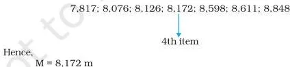
The figure above is NCERT’s own working figure for Example 2.3 — seven Himalayan peak heights arranged in ascending order. The arrangement is the step that makes the median visible: with \(N = 7\), the \((7+1)/2 = 4\)th value of this sorted list is the median. Arranging data before finding the median is not optional; it is the definition of the method.
Grouped data — the median formula. When scores are grouped you cannot pick out a middle item, so the chapter gives a formula (NCERT, p. 18):
\[ M = l + \frac{i}{f} \left( \frac{N}{2} – c \right) \]
| Symbol | Meaning |
|---|---|
| \(M\) | Median for grouped data |
| \(l\) | Lower limit of the median class |
| \(i\) | Interval (class width) |
| \(f\) | Frequency of the median class |
| \(N\) | Total number of frequencies or observations |
| \(c\) | Cumulative frequency of the pre-median class |
In words, the formula says: start at the lower edge of the median class, then walk inwards by the fraction of the class width needed to reach the middle observation.
The gap \((N/2 – c)\) counts how many observations are still needed after all the classes before the median class; multiplying by \(i/f\) converts that count of observations into distance along the class.
Memory aid for the six symbols: the mnemonic “My Little Indians Follow Nice Customs” fixes the order — \(M\) is the Median you are finding, \(l\) is the Lower limit, \(i\) the Interval, \(f\) the Frequency of the median class, \(N\) the total, and \(c\) the Cumulative frequency that comes before.
Worked example. The distance of 50 villages from the nearest town (in km) is grouped as follows:
| Distance (km) | Frequency (f) | Cumulative frequency (F) |
|---|---|---|
| 0–10 | 4 | 4 |
| 10–20 | 8 | 12 |
| 20–30 | 10 | 22 |
| 30–40 (median class) | 12 | 34 |
| 40–50 | 10 | 44 |
| 50–60 | 6 | 50 |
- Step 1: Find \(N/2 = 50/2 = 25\).
- Step 2: Count down the cumulative frequency column until the first value greater than 25.
That value is 34, in the class 30–40, so 30–40 is the median class.
- Step 1: Read off the symbols: \(l = 30\), \(i = 10\), \(f = 12\), \(c = 22\) (cumulative frequency of the class just before the median class).
- Step 2: Substitute into the formula.
\[ M = 30 + \frac{10}{12}(25 – 22) = 30 + \frac{5}{6} \times 3 = 30 + 2.5 = 32.5\ \text{km} \]
Final answer: median distance = 32.5 km — half the villages are within 32.5 km and half are farther.
The Mode: The Value That Appears Most Often
The mode is the value with the maximum occurrence or frequency in a data set — the value that appears most often. It is symbolised as \(Z\) or \(M_0\), and NCERT notes it is less widely used than the mean and the median. (NCERT, p. 20) Ungrouped data — inspect, do not calculate.
The chapter gives no mode formula, and that is itself a common point of confusion: the mode is found by inspection of frequency, not by arithmetic. Take daily rainfall (in mm) at ten stations: 42, 39, 42, 41, 38, 42, 40, 37, 39, 40. Arranged in ascending order: 37, 38, 39, 39, 40, 40, 41, 42, 42, 42.
- Step 1: Arrange the values in ascending or descending order.
- Step 2: Count the frequency of each value.
Here 42 occurs three times; no other value occurs more than twice.
Final answer: mode = 42 mm. Because exactly one value has the highest frequency, the series is unimodal.
The chapter’s vocabulary for multiple modes (NCERT, p. 20): two values with equal highest frequency make a series bimodal; three make it trimodal; several make it multimodal; and when no value repeats at all, the series is without mode. The distinction matters for the exam: a bimodal series still has modes — “without mode” means literally no repeated value.
Mean, Median and Mode Compared: The Normal Curve
The comparison of the three measures is done through the normal curve — the bell-shaped frequency curve in which most observations lie on and around the middle, and extreme values are rare. (NCERT, p. 21) Its key property for this chapter: because the curve is symmetrical, the mean, median and mode are the same score.
When data are skewed or distorted in some way, the three measures no longer coincide. (NCERT, p. 21) That separation is the subject of the figure walkthrough below and of Exercise 3(i). Which measure suits which data is decided by each measure’s properties — the reasoning Exercise 3(ii) asks you to give.
| Measure | What it is | Property that decides its use | Geography data it fits best |
|---|---|---|---|
| Mean | Sum of all values ÷ number of observations | Uses every observation; a single extreme value pulls it | Regular data, e.g. average annual rainfall or mean temperature of a region |
| Median | Middle value of the arranged series | Positional; extreme values do not affect it | Data with a few unusually high or low values, e.g. land holding or income across villages |
| Mode | Most frequent value | Found by frequency, not calculation; gives the typical case | Frequency data, e.g. the most common soil type, commonest wage rate or dominant wind direction |
Figure Walkthrough: Normal Curve, Positive Skew and Negative Skew
These three figures are the working framework for Exercise 3(i). Learn them as a set: the normal curve is the symmetrical baseline, and the two skews are what happens when the symmetry breaks.
Fig 2.1 — The Normal Distribution Curve
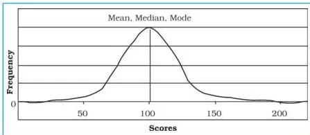
The curve above is symmetrical and bell-shaped: most scores cluster around the middle, and very high and very low scores are rare. Because of that symmetry, the mean, median and mode are the same score — in NCERT’s figure, a score of 100 sits at the centre.
(NCERT, p. 21) NCERT notes that many human traits — intelligence, personality scores and student achievements — have normal distributions. (NCERT, p. 21) The highest point of the curve is where the most frequent score lies, which is by definition the mode; the symmetry places the median and the mean at that same point.
Fig 2.2 — Positive Skew
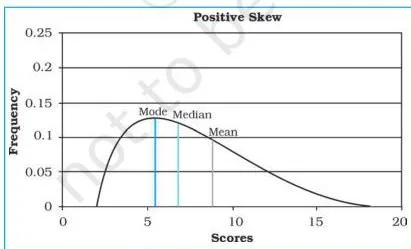
In a positive skew the distribution is no longer symmetrical — the long tail extends toward the higher values. Because the arithmetic mean is an average of every observation, it is dragged farthest in the direction of the tail, so the mean lies beyond the median, which lies beyond the mode.
NCERT’s text states only that in skewed data the three measures do not coincide (NCERT, p. 21); the ordering mean beyond median beyond mode is the standard reading that Exercise 3(i) expects you to state.
Fig 2.3 — Negative Skew
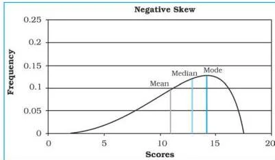
Negative skew is the mirror image: the long tail runs toward the lower values, so the mean is pulled below the median, which is below the mode. (NCERT, p. 22) The one-sentence memory hook for both figures: the mean always follows the tail.
In a positive skew the tail is on the high side and the mean is the largest of the three; in a negative skew the tail is on the low side and the mean is the smallest.
Definitions: The Terms You Need for Data Processing
Use this table when a term stops you mid-calculation — each entry gives the plain meaning and the NCERT page where the term is used.
| Term | Meaning in one line | NCERT page |
|---|---|---|
| Measures of central tendency | Statistical techniques that find the centre of a distribution — the representative value of the whole set | p. 12 |
| Statistical average | Another name for a measure of central tendency | p. 12 |
| Mean | Sum of all values divided by the number of observations; the arithmetic average | p. 14 |
| Median | The middle-ranking value of an arranged series; a positional average written \(M\) | p. 18 |
| Positional average | An average that depends on the position of a value in the ordered series, not its size | p. 18 |
| Mode | The maximum occurrence or frequency at a particular value; written \(Z\) or \(M_0\) | p. 20 |
| Coding | Reducing large observations by subtracting a constant (the assumed mean) from each | p. 15 |
| Assumed mean | A constant chosen near the centre of the data, subtracted during coding; written \(A\) | p. 15 |
| Deviation | The difference between a score and the assumed mean; written \(d\) | p. 17 |
| Midpoint | The average of the two limits of a class interval, standing in for all values in that class | p. 16 |
| Class interval | A group into which scores are collected, such as 50–70 | p. 16 |
| Cumulative frequency | The running total of frequencies as you move down the classes; written \(F\) or \(c\) | p. 18 |
| Normal curve | A symmetrical, bell-shaped frequency curve with most scores around the middle | p. 21 |
| Positive skew | A frequency curve with a long tail toward higher values | p. 21 |
| Negative skew | A frequency curve with a long tail toward lower values | p. 22 |
| Unimodal / bimodal / trimodal / multimodal | One, two, three or many values sharing the equal highest frequency | p. 20 |
| Without mode | A series in which no value is repeated | p. 20 |
Common Mistakes in Mean, Median and Mode Calculations
These are the slips that cost marks in calculation questions, each tied to the NCERT page where it can happen. Read the first column before you start an exercise.
| The mistake | The correct rule | How to check your answer |
|---|---|---|
| Using \(N/2\) as the rank in the ungrouped median instead of \((N+1)/2\) (p. 18) | The median is the \((N+1)/2\) th item of the arranged series | Count off the middle value; it must have equal numbers of values on both sides |
| Forgetting to arrange the data before finding the median or mode (pp. 18, 20) | Always sort ascending or descending first | Ask: is this list ordered? If not, sort; the median and mode become obvious |
| Using raw class limits instead of midpoints as \(x\) in the grouped mean (p. 16) | \(x\) = midpoint of each class, e.g. 15 for the class 10–20 | Recompute one \(fx\) cell: it must be (lower + upper) ÷ 2 × \(f\) |
| Taking \(c\) as the median class’s own cumulative frequency (p. 18) | \(c\) = cumulative frequency of the class just before the median class | Check \(c\) is smaller than \(N/2\); if \(c \geq N/2\), the wrong class was chosen |
| Adding positive and negative \(fd\) values in a single sum (p. 17) | Add positives and negatives separately, take the absolute difference, keep the sign of the larger sum | A huge \(\sum fd\) usually means a sign slip; a small one confirms the assumed mean was well chosen |
| Choosing an assumed mean far from the centre of the series (p. 17) | Pick \(A\) near the middle — preferably the midpoint of a central class | If the coded deviations \(d\) are all large, shift \(A\) toward the centre |
| Declaring a bimodal series “without mode” (p. 20) | “Without mode” means no value repeats at all; two equal highest frequencies = bimodal | Count the frequency of every value; the mode is any value with the maximum frequency |
| Taking the median of an even-numbered series without averaging the two middle values (p. 18) | For even \(N\), the median is the average of the two middle values | If \(N\) is even, check that you added the two middle values and divided by 2 |
Exam Notes: What NCERT’s Exercises Actually Test
The chapter closes with exercises and an activity on NCERT page 22. None is a trick — each question tests one specific idea of the chapter, and this map tells you which.
| Exercise | The chapter idea that answers it |
|---|---|
| Exercise 1, choose-the-correct-answer (i) | The median is positional and independent of actual values (p. 18) — extreme values cannot move it, so the answer is the median |
| Exercise 1, choose-the-correct-answer (ii) | The mode is the maximum frequency value (p. 20) — the hump is where frequency is highest, so the mode always coincides with it |
| Exercise 2 (i): define the mean | The definition on p. 14 — sum of all values divided by the number of observations; give the formula \(\bar{X} = \sum x / N\) as well |
| Exercise 2 (ii): advantages of the mode | The mode identifies the most frequently occurring value, so it points to the most common observation; it is found by frequency, not calculation (p. 20) |
| Exercise 3 (i): relative positions with diagrams | The normal curve (all three measures coincide) and the two skews (the mean follows the tail) — draw Figs 2.1–2.3 and label mean, median and mode on each |
| Exercise 3 (ii): applicability of mean, median and mode | From their merits and demerits: the mean uses every value but is pulled by extremes; the median resists extremes but ignores actual magnitudes; the mode gives the typical value but may be absent or multiple |
The Activity (p. 22) asks for an imaginary geographic example computing the ungrouped mean by both direct and indirect methods. A working template: suppose six stations record annual rainfall (mm) as 720, 810, 690, 760, 830 and 705.
Direct: \(\sum x = 4515\), so \(\bar{X} = 4515/6 = 752.5\ \text{mm}\).
Indirect: choose \(A = 700\); deviations \(d\) are 20, 110, −10, 60, 130, 5, with \(\sum d = 315\).
\[ \bar{X} = A + \frac{\sum d}{N} = 700 + \frac{315}{6} = 700 + 52.5 = 752.5\ \text{mm} \]
Conclusion: both methods agree at 752.5 mm — the indirect route is arithmetic relief, never a different result.
One honest reminder: textbook contents and the examinable syllabus are not always identical — check the current official syllabus for what is examinable this session.
Data Processing Class 12: What to Revise and Remember
A one-read condensation for the night before. This chapter has no printed summary block, so these are the points that matter.
- The chain: the previous chapter organised and presented data; this chapter summarises the whole set into one representative value. (NCERT, p. 12)
- Three techniques exist — central tendency, dispersion, relationship — but this chapter teaches only central tendency. (NCERT, p. 12)
- The mean is \(\sum x / N\) for ungrouped data and \(\sum fx / N\) for grouped data; the indirect routes \(A + \sum d / N\) and \(A \pm \sum fd / N\) must give the same answer. (NCERT, pp. 14–17)
- In grouped data, class midpoints stand in for the lost individual values, and \(N = \sum f\). (NCERT, p. 16)
- The median is the \((N+1)/2\) th item of the arranged series; for grouped data, \(M = l + (i/f)(N/2 – c)\). (NCERT, pp. 18–20)
- The median is positional and extreme-proof — that single property answers Exercise 1(i). (NCERT, p. 18)
- The mode is found by frequency, not calculation; the vocabulary is unimodal, bimodal, trimodal, multimodal and without mode. (NCERT, p. 20)
- In a normal curve all three measures coincide; in skewed data they separate and the mean follows the tail. (NCERT, pp. 20–22)
Related Resources
This listing is maintained for the 2026-27 academic session using the NCERT textbook information available to us. NCERT remains the authority for confirming the latest edition.
If this chapter’s calculations are still unclear, these pages give you the surrounding context.
- Class 12 Geography revision notes — the hub that holds the other chapters of this book.
- The previous chapter, Data: Its Source and Compilation — where data comes from and how it is organised and presented, the step before processing.
- The Class 12 hub — every subject’s notes for Class 12 in one place.
- The full CBSE revision notes index — all classes and subjects.
- The Human Development chapter notes — from the other Class 12 Geography book, useful for a full subject revision.
Sources and Data Verification
This page describes Chapter 2 (Data Processing) of NCERT’s Practical Work in Geography, Part-II for Class 12, NCERT printed pages 12 to 22, in the official NCERT edition published on ncert.nic.in. The page references above point at that edition.
This page covers this one chapter, not the other Class 12 Geography NCERT books. It is maintained for the current session using the NCERT information available to us. NCERT settles textbooks, editions and PDFs; CBSE settles curriculum, syllabus and examinations.
Reference: NCERT Class 12 Geography textbook (Practical Work in Geography, Part-II), chapter 2, official edition on ncert.nic.in.
Frequently Asked Questions
What is data processing in Class 12 Geography?
Data processing is the Class 12 Geography chapter (Chapter 2 of Practical Work in Geography, Part-II) in which a whole data set is summarised into a single representative value using measures of central tendency. After the previous chapter organised and presented data, data processing compresses it further into the mean, median and mode. (NCERT, p. 12)
What is the difference between the direct and indirect method of calculating the mean?
Both give exactly the same answer; they differ in the working. The direct method sums every value and divides by the number of observations. The indirect method first subtracts a constant assumed mean from each value (coding), averages those small deviations, then adds the assumed mean back: \(\bar{X} = A + \sum d / N\).
Use the indirect method when the data set is large and the values are big. (NCERT, pp. 14–15)
How do you find the median of grouped data?
Find \(N/2\), identify the class whose cumulative frequency first exceeds it (the median class), then substitute into \(M = l + (i/f)(N/2 – c)\). Quick example: classes 0–10 with \(f = 2\), 10–20 with \(f = 6\), 20–30 with \(f = 10\), 30–40 with \(f = 2\) give cumulative frequencies 2, 8, 18, 20 and \(N = 20\). \(N/2 = 10\) falls in the class 20–30, so \(l = 20\), \(i = 10\), \(f = 10\), \(c = 8\), and \(M = 20 + (10/10)(10 – 8) = 22\). (NCERT, p. 18)
When should I use the mean, median or mode in geography?
Use the mean for regular data where every observation matters, such as average annual rainfall of a region. Use the median when a few extreme values would distort the average — income or landholding across villages — because the median is untouched by extremes.
Use the mode when you want the most common or typical case, such as the dominant soil type or commonest wage rate. (NCERT, pp. 14, 18, 20)
How does a positive skew differ from a negative skew?
In a positive skew the long tail of the frequency curve extends toward higher values, so the mean lies above the median, which lies above the mode. In a negative skew the tail runs toward lower values and the mean falls below the median, which is below the mode. The memory hook: the mean always follows the tail. (NCERT, pp. 21–22)
Can a data set have more than one mode?
Yes. When two values share the highest frequency the series is bimodal; three make it trimodal; several make it multimodal. A series is called “without mode” only when no value repeats at all — a bimodal series still has modes. (NCERT, p. 20)
Explore Class 12 Geography Books
- Previous: Data — Its Source and Compilation
- Next: Human Development
Related chapters:
- Human Geography
- Population
- The World Population