This is your introduction to linear polynomials class 9 notes page: a tight revision guide to Chapter 2 of the rationalised NCERT Ganita Manjari textbook. It collects the key definitions, the form \( y = ax + b \), linear patterns, linear growth and decay, and straight-line graphs into quick re-read tables.
Three worked examples and an error table show where marks are usually lost. The chapter is idea-light, so these notes stay short: read the definitions table first, then the formula box, then work the examples on paper. The FAQ at the bottom answers the questions students search for most.
Everything here follows the rationalised NCERT Class 9 Mathematics textbook; the official chapter PDF on the NCERT website is the final reference if you wish to verify any definition or formula.
Introduction to Linear Polynomials Class 9 Notes: What This Chapter Covers
The chapter builds one idea on another: name the parts of an algebraic expression, sort expressions by degree, then study the special behaviour of degree-1 (linear) expressions and their graphs. The table shows the order of ideas and where each lives in the textbook.
| Stage | What you learn | NCERT pages |
|---|---|---|
| 1. Naming parts | Terms, variables, coefficients and constants in an algebraic expression | p. 17 |
| 2. Sorting by degree | Univariate polynomials and their four types (constant, linear, quadratic, cubic) | p. 18-19 |
| 3. The linear pattern | Constant difference between consecutive values; the input-output view of a function | p. 20-24 |
| 4. Growth and decay | Modelling situations where a quantity rises or falls by a fixed amount | p. 25-26 |
| 5. Linear relationship | \( y = ax + b \): slope \( a \), y-intercept \( b \), found from two data points | p. 27 |
| 6. Graphs | Plotting straight lines; parallel lines when \( a \) is fixed and \( b \) varies | p. 28-36 |
If the vocabulary feels new, the world of numbers notes cover the number foundations that variables stand for, and the Class 9 Mathematics notes index holds the rest of the chapters.
Important Concepts and Definitions (with Examples)
These are the exact terms of the chapter. Learn them as a family: coefficient and constant are the numbers, variable is the letter, degree is the highest power, and linear means degree 1.
| Term | Meaning | Example |
|---|---|---|
| Algebraic expression | Numbers, variables and operation symbols combined | \( 4x + 5y + 3 \) |
| Term | A part of an expression separated by + or − | Terms of \( 4x + 5y + 3 \) are \( 4x \), \( 5y \), 3 |
| Variable | A letter that stands for a number | \( x, y, m, n \) |
| Coefficient | The number multiplying a variable | In \( 4x \), 4 is the coefficient of \( x \) |
| Constant | A term with no variable | The 3 in \( 4x + 5y + 3 \) |
| Polynomial (univariate) | An algebraic expression in one variable and its powers | \( x^2 + 5x + 1 \), \( 5y^3 + y^2 + 2y – 1 \) |
| Degree | The highest power of the variable in a polynomial | \( x^2 + 5x + 1 \) has degree 2 |
| Linear polynomial | A polynomial of degree 1 | \( 3z + 7 \), \( 2x + 3 \) |
| Constant polynomial | A polynomial of degree 0 | 8, written as \( 8x^0 \) |
| Linear pattern | A sequence where the difference between consecutive terms is constant | 1, 3, 5, 7, 9, … |
| Linear equation | A linear polynomial equated to a constant | \( 2x + 10 = 64 \) |
| Function | A polynomial seen as an input-output process | Input \( x = 4 \) gives output \( 2(4) + 3 = 11 \) |
| Linear relationship | The relation \( y = ax + b \) between two variables | \( y = 20x + 150 \) |
| Slope | The constant increase in \( y \) per unit of \( x \); the \( a \) in \( y = ax + b \) | \( y = 2x – 1 \) has slope 2 |
| y-intercept | The point where a line cuts the y-axis, \( (0, b) \) | \( y = x + 3 \) cuts the y-axis at (0, 3) |
Polynomial types by degree (comparison table)
The degree gives a polynomial its family name. Memorise the four names with one example each.
| Type | Degree | Example | Graph shape |
|---|---|---|---|
| Constant | 0 | 8 (that is, \( 8x^0 \)) | — |
| Linear | 1 | \( 3z + 7 \), \( 2x + 3 \), \( 200 + 50m \) | Straight line |
| Quadratic | 2 | \( x^2 + 5x + 1 \), \( 10x – x^2 \) | — |
| Cubic | 3 | \( 5y^3 + y^2 + 2y – 1 \) | — |
The function idea
A polynomial can be read as an input-output process: feed it a value of \( x \), it returns a value of the expression. The chapter calls this machine a function (NCERT, p. 21).
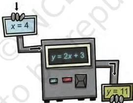
For the linear function \( 2x + 3 \), input \( x = 4 \) gives output \( 2(4) + 3 = 11 \), while \( x = -6 \) gives -9. A quadratic like \( 10x – x^2 \) uses the same machine, but its output changes by a varying amount.
Linear patterns: the constant-difference property
A linear pattern is a sequence where consecutive terms differ by the same number. The tile pattern below grows by two squares at every stage.
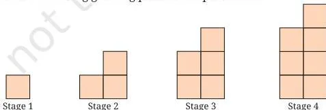
The tile counts 1, 3, 5, 7, 9, … form a linear pattern with constant difference 2, and stage \( n \) holds \( 2n – 1 \) tiles (NCERT, p. 23). Whenever the \( n \)th term of a pattern is a linear polynomial, the pattern is linear.
Key Formulas and Symbol Meanings
Everything in this chapter runs on one skeleton, \( y = ax + b \). The table lists every formula shape you need and what each symbol means.
| Formula | Meaning of symbols |
|---|---|
| \( y = ax + b \) | \( a \) = slope (constant increase per unit of \( x \)); \( b \) = y-intercept (the point where the line cuts the y-axis) |
| \( y = ax \) | Line through the origin (0, 0); the larger \( a \), the steeper the line |
| \( T_n = T_1 + (n-1)d \) | \( T_1 \) = first term, \( d \) = common difference; for the tiles, \( 1 + (n-1) \times 2 = 2n – 1 \) |
| \( y = \text{initial} + \text{rate} \times t \) | Linear growth: quantity rises by a fixed amount, e.g. \( C(d) = 100 + 60d \) |
| \( y = \text{initial} – \text{rate} \times t \) | Linear decay: quantity falls by a fixed amount, e.g. \( h(t) = 3 – 0.5t \) |
| \( a = \dfrac{y_2 – y_1}{x_2 – x_1} \) | Slope from two points \( (x_1, y_1) \) and \( (x_2, y_2) \); substitute one point back to find \( b \) |
Why the constants behave that way
- Slope stays constant because adding 1 to \( x \) adds exactly \( a \) to \( y \). That fixed step is the constant difference of the pattern, and the slope of its line equals that difference (NCERT, p. 32).
- The y-intercept is (0, b) because substituting \( x = 0 \) removes the \( ax \) term, leaving \( y = b \) (NCERT, p. 36).
- Lines with the same \( a \) but different \( b \) are parallel — they tilt identically and only shift up or down (NCERT, p. 36).
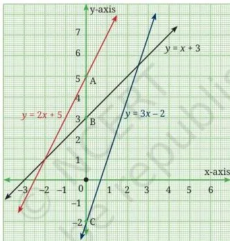
The figure shows the rule in action: the constant term \( b \) is exactly the height at which the line cuts the y-axis.
Fresh analogy: the taxi meter
A linear polynomial behaves like a taxi ride. The flag-down charge is the y-intercept \( b \): you pay it even when the distance \( x \) is zero. The per-kilometre rate is the slope \( a \): each extra kilometre adds exactly \( a \) rupees. Total fare = flag-down + rate \( \times \) kilometres.
Big \( a \) means the meter climbs fast (steeper line); negative \( a \) means the meter runs backwards — that is decay. The chapter’s auto-rickshaw fare, \( 25 + 15(n – 2) \) for \( n \geq 2 \) km, is the same structure with a stepped start (NCERT, p. 24).
Memory device: slope and y-intercept
Slope = mountain steepness. When \( a \gt 1 \) the line climbs steeply, when \( 0 \lt a \lt 1 \) it is gentle, and \( y = ax \) always passes through the origin (NCERT, p. 32). y-intercept = where the line cuts the y-axis. “Intercept” means “cut”: put \( x = 0 \) and the cut point is \( (0, b) \).
For \( y = 3x – 2 \) the cut is 2 units below the origin, so the y-intercept is -2 (NCERT, p. 36).
Worked Examples (Step-by-Step)
Example A: identify the degree and type of a polynomial
Question: For \( 6x^2 – 4x + 9 \), find the degree, the type, and the coefficient of \( x \).
- Step 1: Write every power of \( x \) explicitly: \( 6x^2 – 4x^1 + 9x^0 \).
- Step 2: The powers present are 2, 1 and 0.
- Step 3: The highest power is 2, so the degree is 2.
- Step 4: A polynomial of degree 2 is called a quadratic polynomial.
- Step 5: The coefficient of \( x \) is the number attached to \( x^1 \), which is -4.
Final answer: degree 2, quadratic polynomial, coefficient of \( x \) = -4.
Example B: find the linear relationship from two points
Question: A bill \( y \) (in ₹) depends on data used \( x \) (in GB) through \( y = ax + b \). When \( x = 2 \), \( y = 40 \); when \( x = 6 \), \( y = 80 \). Find \( a \) and \( b \).
- Step 1: Start from the general form \( y = ax + b \).
- Step 2: Substitute (2, 40): \( 40 = 2a + b \).
- Step 3: Substitute (6, 80): \( 80 = 6a + b \).
- Step 4: Subtract the first equation from the second: \( 80 – 40 = (6a – 2a) + (b – b) \), so \( 40 = 4a \), giving \( a = 10 \).
- Step 5: Put \( a = 10 \) into Step 2: \( b = 40 – 2(10) = 20 \).
- Step 6: Write the relationship: \( y = 10x + 20 \).
- Step 7: Verify with the second point: \( 10(6) + 20 = 80 \) ✓.
Final answer: \( y = 10x + 20 \); slope \( a = 10 \) (₹10 per GB) and y-intercept \( b = 20 \) (₹20 fixed charge).
Shortcut check: the slope is \( \dfrac{80 – 40}{6 – 2} = 10 \), the rate of change of \( y \) per unit of \( x \). Always confirm \( b \) by substituting one known point back.
Example C: graph y = 3x + 2
Question: Draw the graph of \( y = 3x + 2 \) and state its y-intercept.
Step 1: Put \( x = 0 \): \( y = 3(0) + 2 = 2 \).
This gives the y-intercept point (0, 2).
- Step 1: Pick a second value, \( x = 1 \): \( y = 3(1) + 2 = 5 \), giving (1, 5).
- Step 2: Plot (0, 2) and (1, 5) on the coordinate plane, join them with a ruler, and extend the line in both directions.
- Step 3: Check with a third point: \( x = 2 \) gives \( y = 8 \), so (2, 8) must lie on your line.
A point lies on the line only if its coordinates satisfy the equation (NCERT, p. 29).
Final answer: slope = 3, y-intercept = 2, and the line cuts the y-axis at (0, 2).
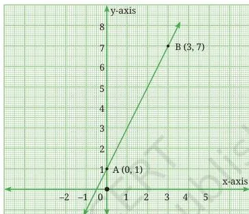
The figure shows the same two-point method on \( y = 2x + 1 \): plot two points, join, extend (NCERT, p. 28-29).
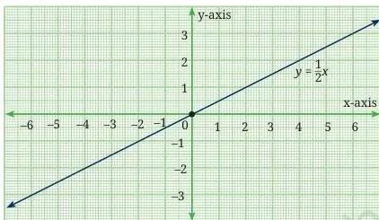
Lines of the form \( y = ax \) all pass through the origin; the larger the slope, the steeper the line (NCERT, p. 31-32).
Honest Common Errors and How to Avoid Them
A few small slips cause most lost marks in this chapter. Each row below is an error, its correction, and a way to check yourself.
| Students write X | Correct is Y, because | How to check your answer |
|---|---|---|
| “The coefficient of \( z \) in \( 4z^3 + 5z^2 – 11 \) is 5.” | It is 0. The \( z \) term is missing, and the polynomial equals \( 4z^3 + 5z^2 + 0z – 11 \). | List all powers from highest to 0; any absent power has coefficient 0. |
| “\( 2x + 10 = 64 \) is a linear polynomial.” | It is a linear equation. The linear polynomial is \( 2x + 10 \); a polynomial never carries an equals sign. | Spot an “=” sign? Then it is an equation, not an expression. |
| “In \( y = 2x + 5 \), the slope is 5 and the y-intercept is 2.” | Slope = 2, y-intercept = 5. The slope \( a \) multiplies \( x \); \( b \) is the constant added alone. | The number stuck to \( x \) is \( a \); what remains when you cover the \( x \)-term is \( b \). |
| “The y-intercept of \( y = 3x + 2 \) is the point (2, 0).” | It is (0, 2). Putting \( x = 0 \) leaves \( y = b \), so the line cuts the y-axis at (0, \( b \)). | The y-intercept point always has x-coordinate 0. |
| “\( y = -3x \) grows just like \( y = 2x \).” | \( y = 2x \) grows (positive slope) but \( y = -3x \) decays (negative slope). | Test two inputs: if \( y \) falls as \( x \) rises, the slope is negative. |
Misconception autopsy: polynomial vs equation
The mix-up happens because word problems end in an equation. Watch the sequence in the chapter: \( 2x + 10 \) is a linear polynomial; equating it to 64 gives the linear equation \( 2x + 10 = 64 \) (NCERT, p. 20-21).
A polynomial is an expression — a value that changes with \( x \). An equation is a condition: a true/false statement that pins \( x \) down. The same polynomial can sit inside many equations, so never add an equals sign when a question asks for the polynomial.
Natural Patterns in the Board Examination
Based on CBSE question patterns in this chapter — not a year-specific prediction — questions recur in a few shapes:
- Identification: degree, type, or coefficient of a term, including missing terms whose coefficient is 0 (Exercise 2.1 style).
- Evaluation: substitute a value into a polynomial and simplify (Exercise 2.2 style).
- Word problems: form a linear polynomial, equate it, and solve — age, coin and money problems (Exercise 2.2 and end-of-chapter style).
- Growth/decay from a table: state whether the fixed change is positive (growth) or negative (decay) (Exercise 2.4 style).
- Linear relationship from two data points: when a table of \( x \) and \( y \) is given, calculate slope as \( \Delta y / \Delta x \), then find \( b \) (Exercise 2.5 style).
- Graph questions: complete a table of points, plot them, draw the line, and read off slope and y-intercept (Exercise 2.6 style).
For a full-marks graph answer: write the equation, list the plotted points, draw the line, then state the slope and the y-intercept separately with the exact cutting point (0, \( b \)). Plotting builds on the coordinate plane — revise our coordinate geometry notes if the axes feel shaky, and browse the Class 9 notes hub for the other chapters.
Quick Revision Recap (One-Page Memory Aid)
Polynomial types cheat sheet
| Type | Degree | Example | Graph (studied in this chapter?) |
|---|---|---|---|
| Constant | 0 | 8 | — |
| Linear | 1 | \( 2n – 1 \) | Straight line |
| Quadratic | 2 | \( 10x – x^2 \) | — |
| Cubic | 3 | \( 5y^3 + y^2 + 2y – 1 \) | — |
Growth vs decay at a glance
| Behaviour | Slope sign | What happens | Example |
|---|---|---|---|
| Linear growth | Positive (\( a \gt 0 \)) | Quantity increases by a fixed amount each step | \( y = 2x + 3 \), \( C(d) = 100 + 60d \) |
| Linear decay | Negative (\( a \lt 0 \)) | Quantity decreases by a fixed amount each step | \( y = -5x + 1 \), \( h(t) = 3 – 0.5t \) |
Reading \( y = ax + b \) quickly: \( a \) = slope = constant difference between consecutive terms; \( b \) = y-intercept = cut point (0, \( b \)); fixed \( a \) with varying \( b \) gives parallel lines. The input-output view (function) is the heart of the chapter — every linear pattern is a machine with a constant step.
Real-life application: battery drain as linear decay
Suppose your phone starts at 100% and drains a fixed 10% every hour. The remaining charge is \( b(t) = 100 – 10t \), a linear decay model because the slope -10 is negative. After 4 hours: \( 100 – 10(4) = 60\% \). It reaches zero when \( 100 – 10t = 0 \), that is, after 10 hours.
Any situation where a starting amount changes by a fixed amount per unit time — data balance, water level, phone value — uses the same \( y = \text{initial} \pm \text{rate} \times t \) structure.
Carry one sentence into the exam: a linear polynomial is a function \( y = ax + b \) whose output changes by the fixed amount \( a \) for every 1-unit change of input; the sign of \( a \) decides growth or decay, and \( b \) anchors the line at (0, \( b \)).
For the rest of the syllabus, the all CBSE notes pages keep every chapter in one place.
Frequently Asked Questions
How do you calculate the degree of a polynomial?
Look at the highest power of the variable. In \( 4x + 1 \) the highest power is 1 (since \( 4x = 4x^1 \)), so the degree is 1. In \( 6x^2 – 4x + 9 \) the highest power is 2, so the degree is 2.
How can we decide if a polynomial is linear?
A polynomial is linear when its degree is exactly 1, meaning the variable appears only to the first power. So \( 3z + 7 \), \( 2x + 3 \) and \( 5 – 4y \) are linear, while \( x^2 + 1 \) is not.
What are growth and decay in the context of linear polynomials?
Linear growth is a pattern where a quantity increases by a fixed amount over equal intervals — positive slope, like \( y = 100 + 60d \). Linear decay is a pattern where a quantity decreases by a fixed amount — negative slope, like \( y = 3 – 0.5t \).
How to plot the graph of a linear polynomial using two points?
Put \( x = 0 \) to get the y-intercept point (0, \( b \)), then choose a second convenient \( x \) and compute \( y \). Plot both points, join them with a ruler, and extend the line in both directions. A third point should land on the same line.
What does the relationship between slope and the constant difference represent in a linear sequence?
In a linear pattern the difference between consecutive terms is a fixed number, and the slope of the line representing the pattern equals that number. For the tiles 1, 3, 5, 7, … the difference is 2 and the line \( y = 2n – 1 \) has slope 2.
Reference: NCERT Class 9 Mathematics textbook (Ganita Manjari), chapter Introduction to Linear Polynomials.
Explore Class 9 Mathematics Notes
- Class 9 Maths Notes
- Class 9 CBSE Notes
- CBSE Notes for Classes 1 to 12
- Previous: Orienting Yourself: The Use of Coordinates
- Next: The World of Numbers
Related chapters:
- Exploring Algebraic Identities notes
- I'm Up and Down, and Round and Round notes
- Measuring Space: Perimeter and Area notes